
This post is a brief description of my findings on setting up Geoserver from scratch and some particular points on setting it up for an Oracle connection. I hope it will prove useful for others.
INSTALLATION
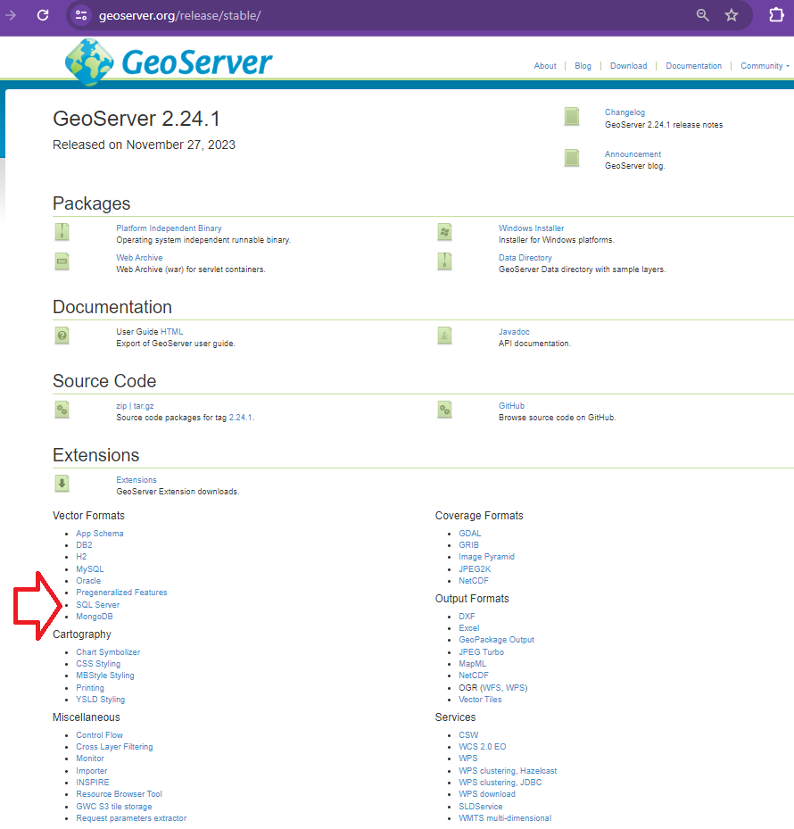
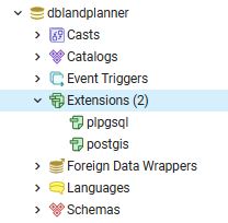
GeoServer with ORACLE database connection support
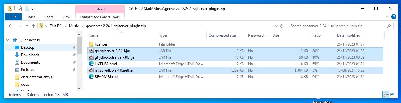
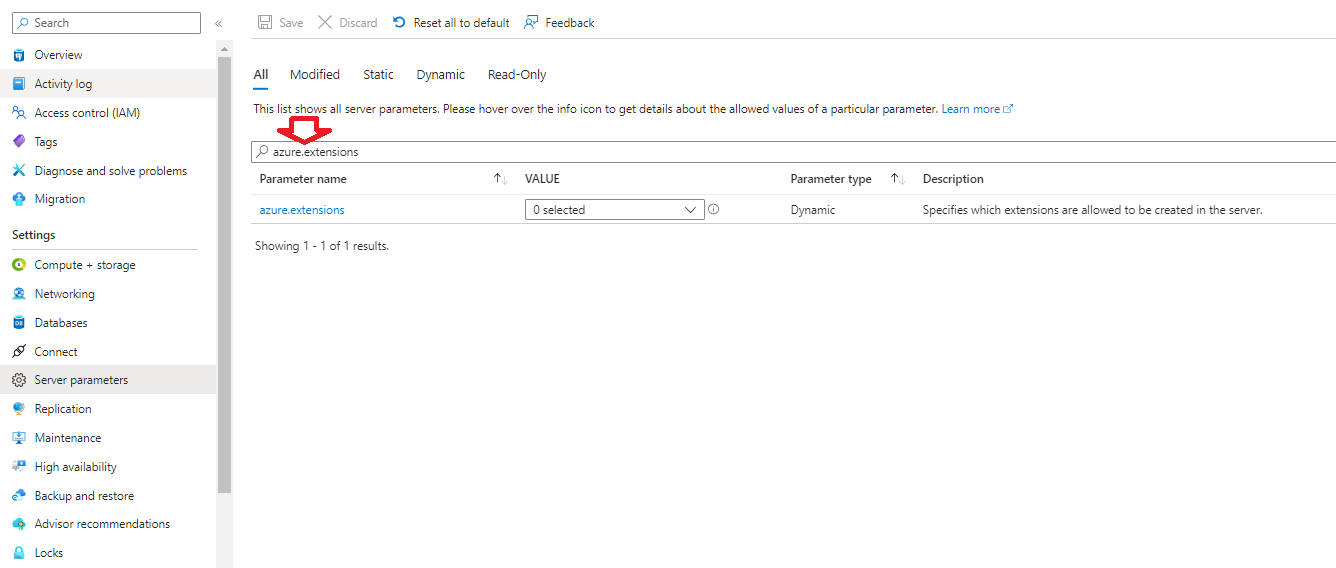
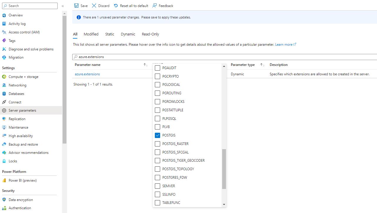
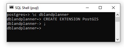
Geoserver Postgres (PostGIS) connection support comes with the default installation. This is NOT the case for Oracle or SQL Server therefore for enterprise purposes it is a requirement to install Geoserver WITH Oracle and SQL Server extensions if you wish to support these database connections.
I’ve done a post on Geoserver on windows installation link here that talks specifically about SQL Server. I will not go into a lot of detail about installation here. See below for links to the geoserver docker image I didn’t install the geoserver I describe here but I can confirm that we have been successful in including Oracle as a plugin to our Geoserver installation and we are able to connect.
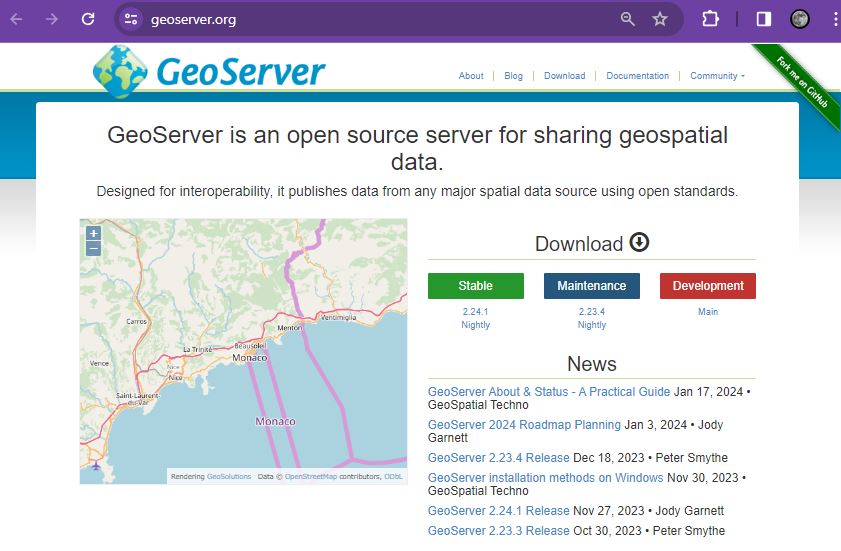
Official Geoserver Docker Image GITHUB
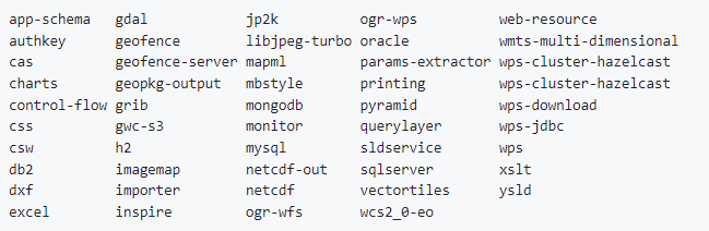
Below is a recent (Feb 2024) list of Docker parameters available at install including Oracle and SQL Server please seek advice on the use of Docker for installation if you are not familiar with it already.
GENERAL SETUP
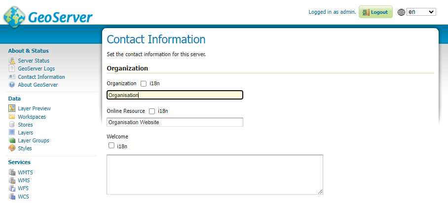
Contact Information – General Setup
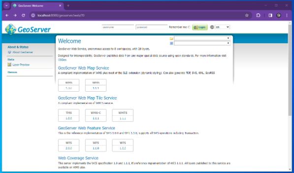
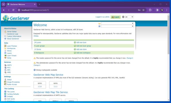
On the Welcome screen there is a line that reads For more information visit {organization} to change this from the initial meaningless variable setting go to Contact Information and fill out your organisation.
Difference between Save and Apply – General point

In geoserver admin there are a lot of pages where there is a Save and an Apply button. Most users initially at least find this confusing.
In GeoServer, the terms “Save” and “Apply” serve different purposes:
Save:
When you click “Save”, it permanently stores the changes you’ve made to the configuration. These changes are saved in the GeoServer configuration files. , “Save” ensures that your modifications persist even after restarting GeoServer or rebooting the system. It’s like committing your changes to a version control system—it makes them permanent.
Apply:
“Apply”, on the other hand, is more immediate. When you click “Apply”, it takes the current configuration (including any unsaved changes) and applies it dynamically. The applied changes take effect immediately without requiring a restart or permanent storage. Think of it as a temporary adjustment that affects the running instance of GeoServer but doesn’t alter the saved configuration. In summary, “Save” makes changes permanent, while “Apply” applies them immediately without saving them to the configuration files
![]()
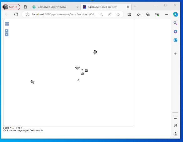
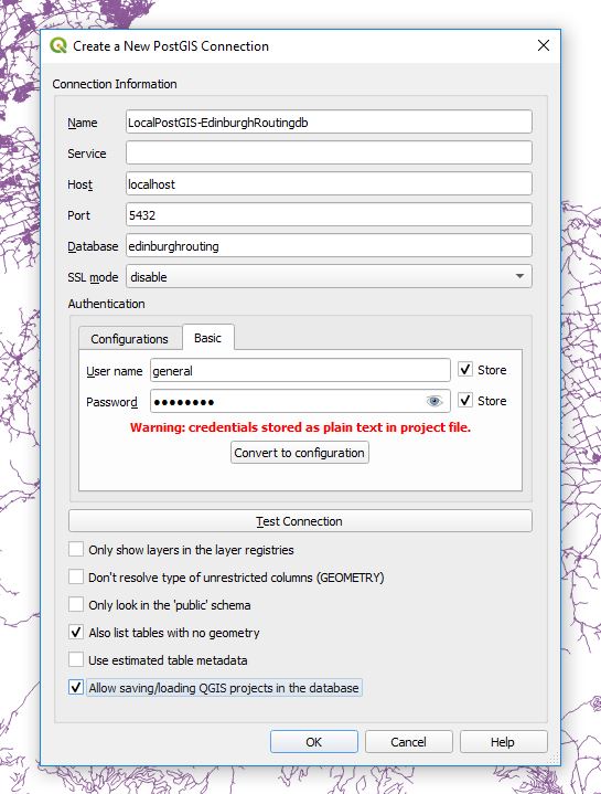
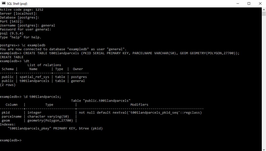
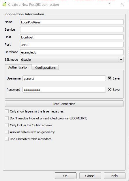
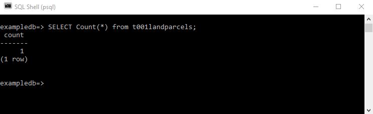
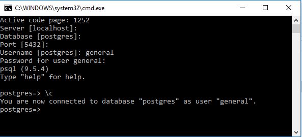
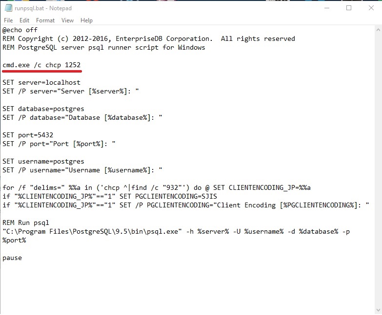
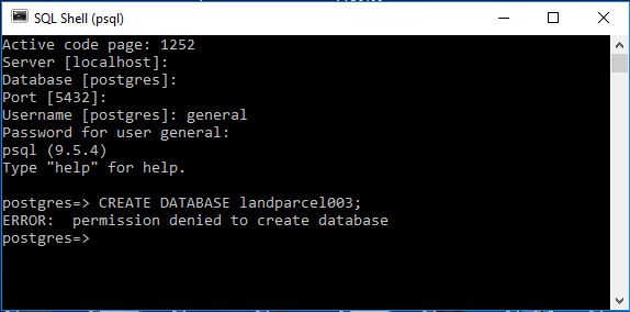
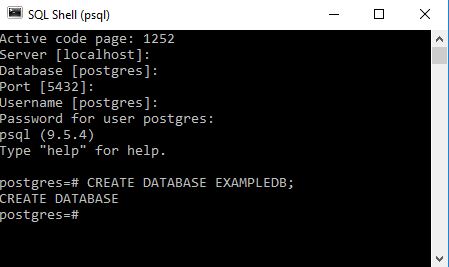
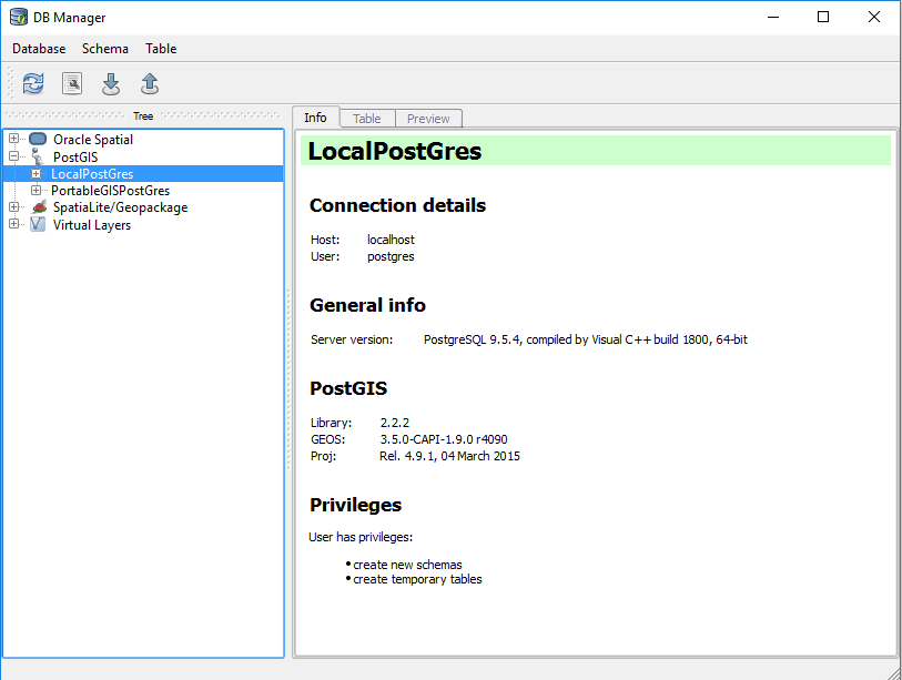
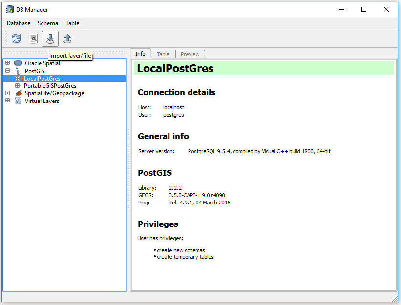
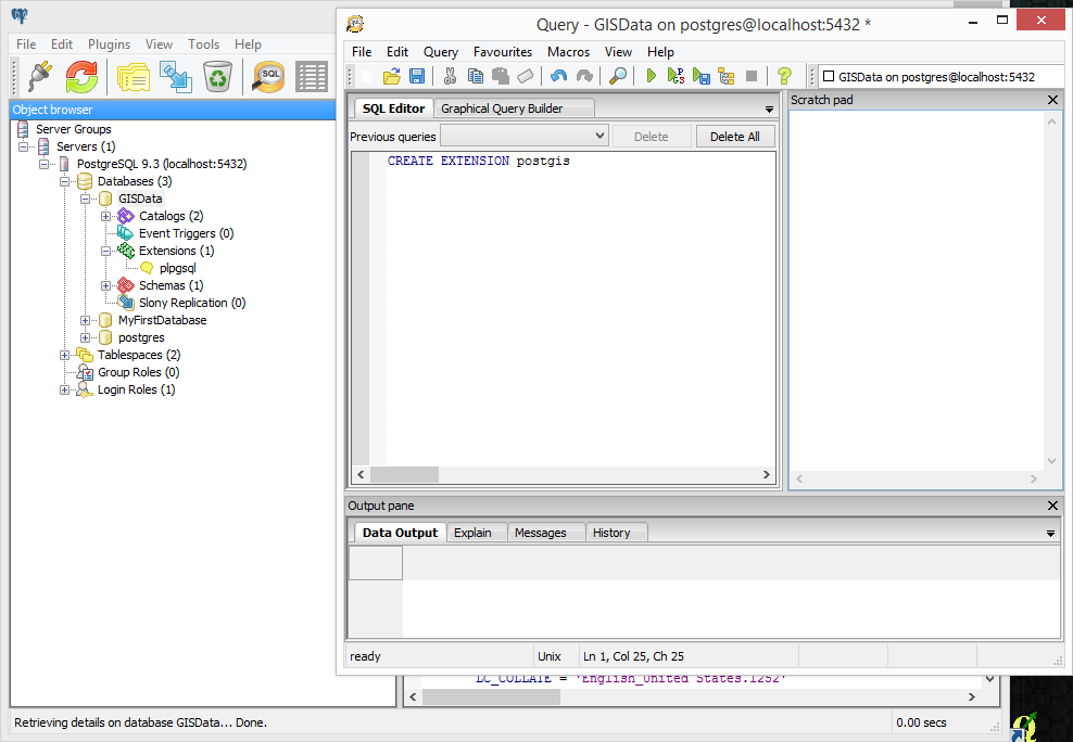
The first thing you will want to do is determine if you can actually connect to your ORACLE database.
ORACLE required parameters for database connection. Before you continue make sure you have the following
ORACLE host name
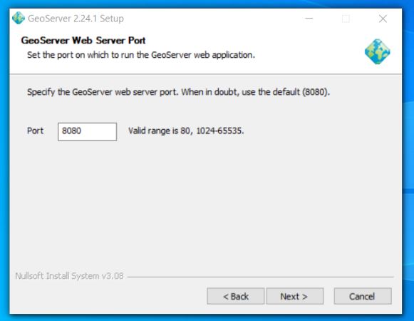
Port ORACLE database (default 1521)
database name
user – case sensitive
password – case sensitive
Geoserver installed with Oracle extension
It is good idea to get your DBA to setup a read only user if you are connecting to a database that is part of a vendor supplied product as you really should not be editing the database through anything except the vendor’s UI and Geoserver can be setup to allow edit of data. Geoserver has powerful security configuration included but conflicting settings can arise that may alter the intended security levels making it safer to enforce read only least privilege at the database level.
ORACLE and Postgres – some SQL Differences
Please be aware Oracle databases are by default case sensitive but may convert SQL Strings to upper case when passed to Oracle. I believe this complies strictly with the SQL Standard.
Postgres classifies tables, columns views and other database objects as Identifiers. SQL Identifiers must begin with a letter. If possible avoid including special characters in the naming of identifiers because although postgres may support them special characters are not allowed in the SQL Standard so their use might render applications less portable. Additional identifiers and keyword must begin with a letter. Keywords are defined as items such as SELECT / UPDATE / CREATE etc.. The SQL Standard says that databases should not define a key word that contains a digit or starts or ends with an underscore so identifiers could be something like t001users should be safe against possible conflict with future extensions of the standard. In postgres the maximum identifier length is 63 bytes. Additionally Postgres also folds unquoted names to lower case but some postgres management UIs allow for the naming of identifiers with varied case.
UPSHOT for Geoserver (and anything else for that matter)
If you are having difficulty referencing tables or views in any enterprise database – experiment with the case sensitivity in the query. There might be some folding of object names when passed to the server.
This characteristic should be born in mind when using SQL Views in Geoserver.
ORACLE Store setup to get the most out of Geoserver
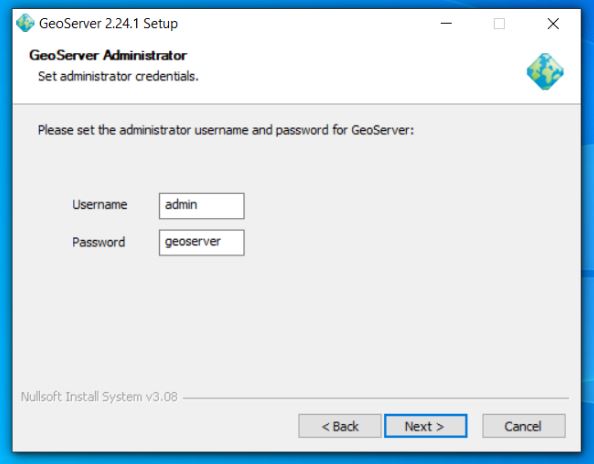
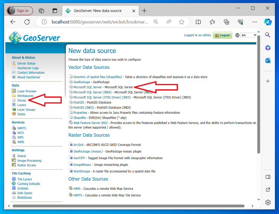
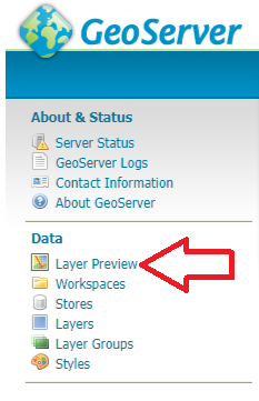
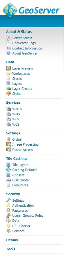
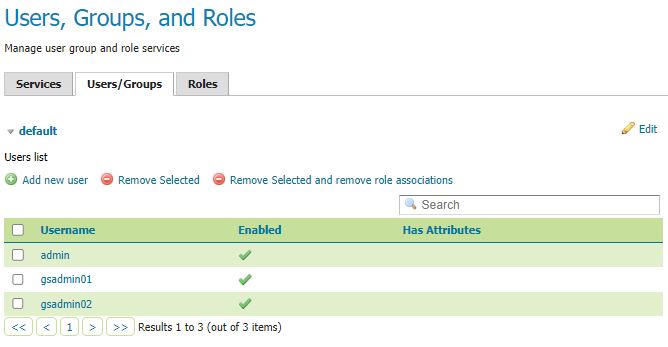
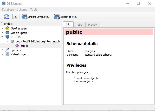
Login to Geoserver admin panel using your admin account
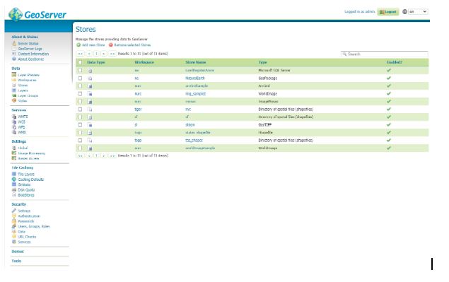
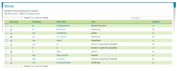
On the left hand side under Data hit Stores
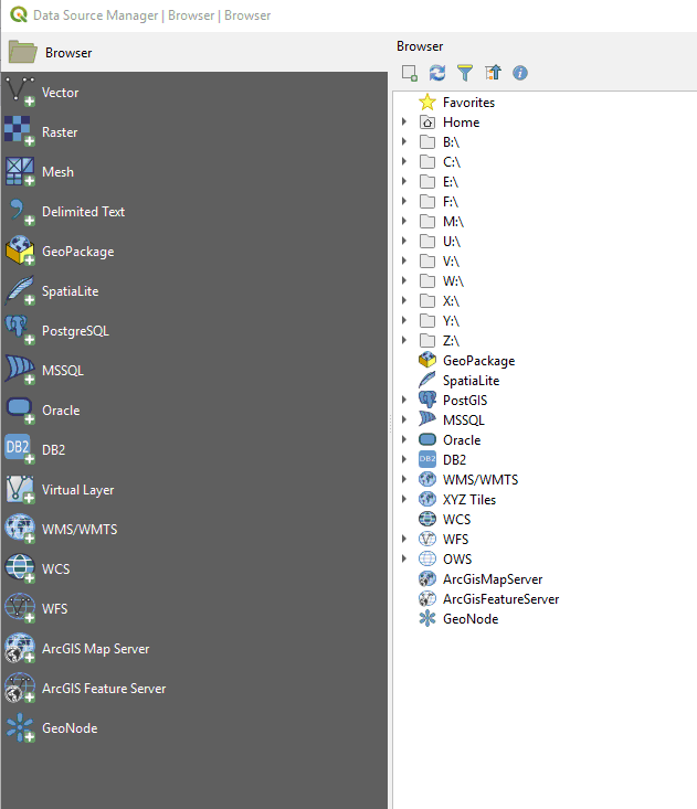
Assuming you have successfully installed Geoserver with the Oracle extension you should be presented with the following dialog and in particular the items highlighted below.
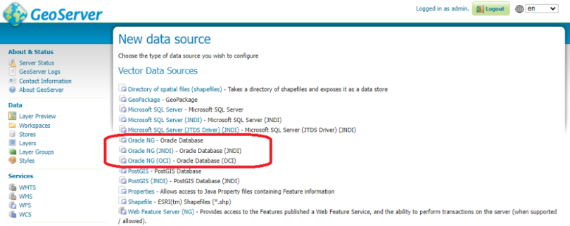
Oracle NG uses a standard Oracle driver (ignore the other options this article will not explain them)
Select Oracle NG
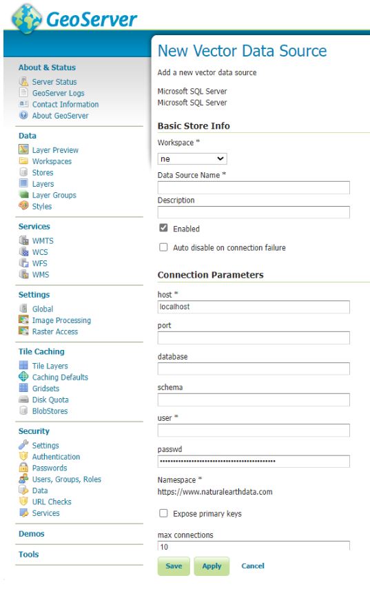
Use the default settings for most things but IMPORTANTLY ensure Expose Primary Keys is ticked
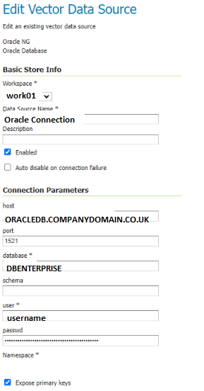
NOTE from our brief testing we found that exposing primary keys seemed to be one factor that improved stability in our Oracle connection when dealing with QGIS.
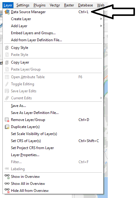
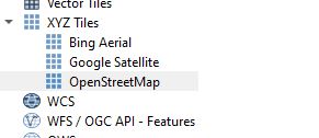
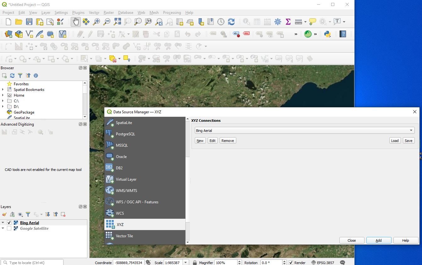
QGIS WFS set up to improve Oracle Connection Stability
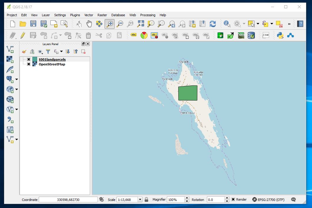
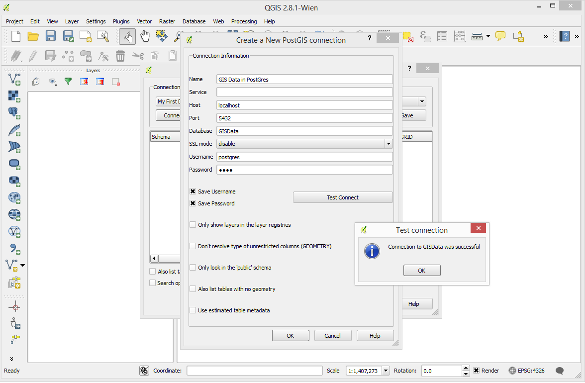
It is recommended that you have a copy of QGIS to test setup to things like WFS
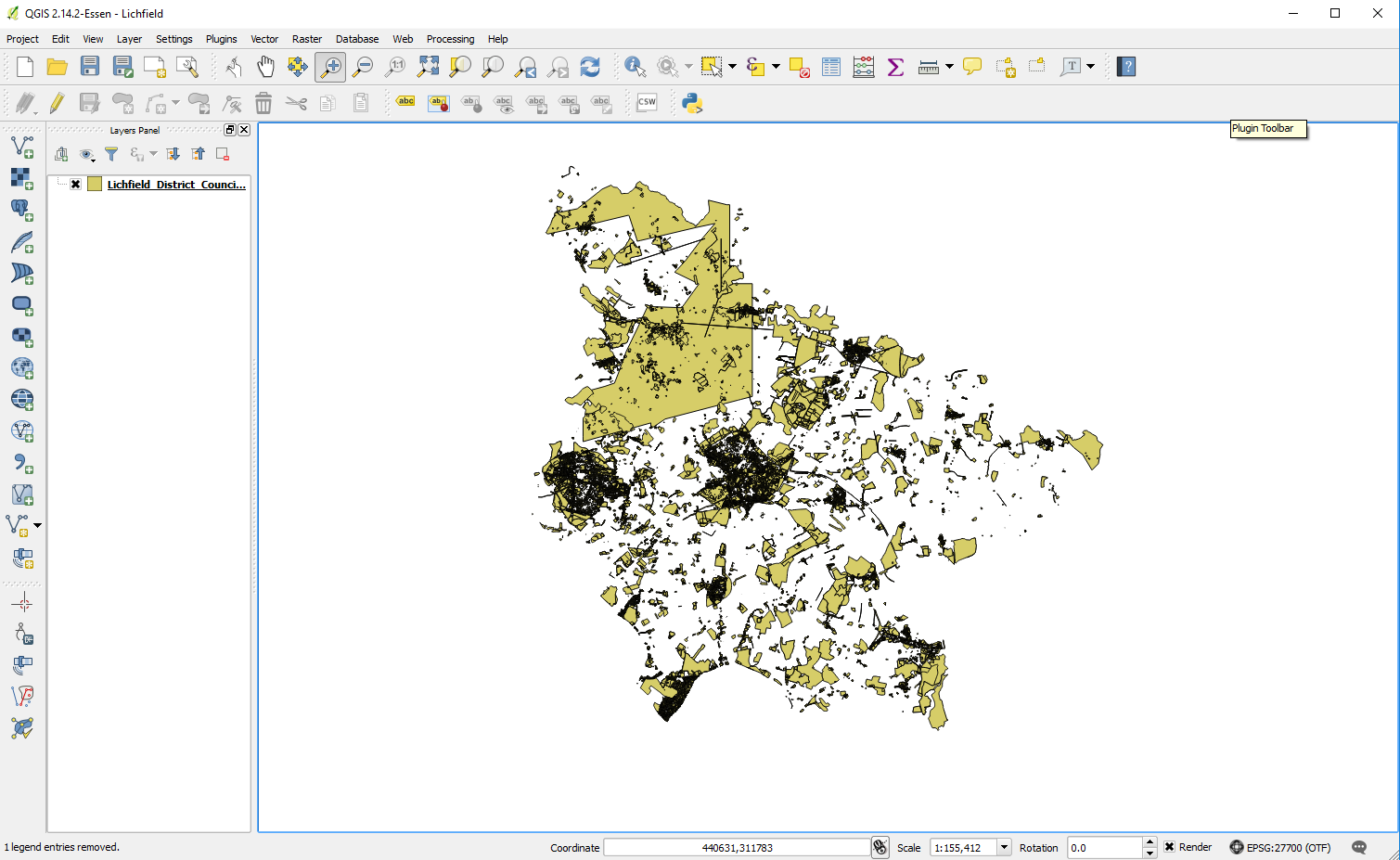
When we first started displaying specifically the Oracle spatially enabled table in QGIS via WFS service we found that the layer would initially display but if we were to leave the project and go back in for a period of time the layer would not be visible. This seemed to be temporary and after an unpredictable amount of time the layer would reappear. The attribute table continued to be viewable but polygons were not visible.
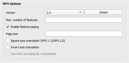
We fixed this by ensuring Expose Primary Key (see Geoserver layer configuration) was ticked and within QGIS within the WFS Connection Configuration ensure within the WFS options section that the version is set to match the linked WFS Service. This might not be necessary in all QGIS versions.
LAYER Config
Useful background information (partly written by co-pilot)
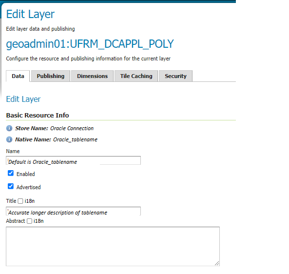
Enabled and Advertised parameters – Layer Config
In GeoServer, the Enabled and Advertised checkboxes play distinct roles in layer configuration:
Enabled:
When a layer is enabled, it means that the layer is available for requests (such as WMS GetMap or WMS GetFeature). If a layer is not enabled, it won’t be accessible for any kind of request. However, it will still appear in the configuration (and in the REST config). Essentially, enabling a layer makes it operational and ready to serve data.
Advertised:
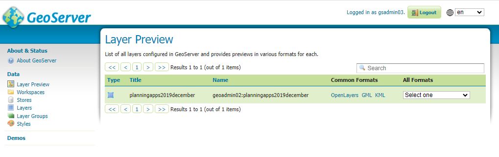
By default, a layer is advertised. An advertised layer is included in the GetCapabilities request and appears in the layer preview. However, if you uncheck the Advertised checkbox, the layer will still be available for data access requests (like WMS), but it won’t appear in any capabilities documents or previews. In other words, non-advertised layers remain functional but are not explicitly listed in service metadata. Remember, enabling a layer makes it operational, while advertising it determines whether it appears in service capabilities and previews
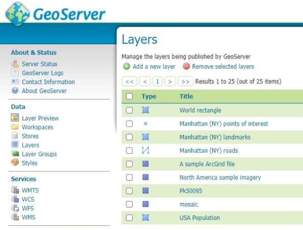
Name and Title parameters – Layer Config
Name:
The Name corresponds to the identifier used to reference the layer in WMS (Web Map Service) requests. It is primarily used for computer interaction and serves as an internal reference default name is usually the name of the table or the name of the referenced view. When creating a new layer for an already-published resource, the Name must be unique to avoid conflicts. Essentially, it’s the technical name associated with the layer.
Title:
The Title provides a human-readable description that briefly identifies the layer to clients. Unlike the Name, which is for computers, the Title is meant for humans to read. It helps users understand the purpose or content of the layer. For example, if you have a layer representing a map of the USA, you might set the Title to “This is a map of USA.” Remember, while the Name is essential for system functionality, the Title enhances user experience by providing meaningful context about the layer1
Security – the Name does not need to be the table or view name you are referencing. This string appears in the URL which may be viewable to the user – you may wish to obfuscate this by changing the name
i18n – Internalization – Layer Config
Internationalization (i18n):
GeoServer supports returning a GetCapabilities document (used for describing available services and layers) in various languages. The i18n functionality is available for the following services:
WMS 1.1 and 1.3
WFS 2.0
WCS 2.0
The i18n editor allows you to provide translations for the title and abstract of various components:
Layers configuration page
Layergroups configuration page
WMS, WFS, and WCS service configuration pages
Additionally, for Styles, there’s a separate i18n configuration (see i18N in SLD).By default, the i18n editor is disabled and can be enabled via the i18n checkbox.
GetCapabilities Document Language:
The language of the GetCapabilities document can be selected using the AcceptLanguages request parameter.GeoServer’s response varies based on the following rules:
Internationalized elements include titles, abstracts, and keywords.If a single language code is specified (e.g., AcceptLanguages=en), GeoServer tries to return content in that language.If multiple language codes are specified (e.g., AcceptLanguages=en,fr), GeoServer attempts to return content in one of the specified languages.
Coordinate Reference Systems – Declared SRS and SRS handling – Layer Config
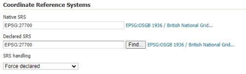
If you are in the UK ensure that Declared SRS is set to 27700
SRS Handling
In GeoServer, the SRS handling setting plays a crucial role in how coordinate reference systems (CRS) are managed. Let’s explore its significance:
Declared SRS:
The Declared SRS specifies the coordinate system that GeoServer publishes to clients. It represents the CRS that clients should use when interacting with the layer. Essentially, it’s the officially declared CRS associated with the layer.
SRS Handling:
The SRS Handling option determines how GeoServer should handle projection transformations when the declared CRS and the native CRS of the data differ. Here are the possible values for SRS Handling:
Force declared (default): In this mode, GeoServer forces the declared SRS upon the data, overwriting the native CRS if necessary.
Other options (not mentioned in the snippet):
Reproject native to declared: GeoServer performs a reprojection from the native CRS to the declared CRS.
Reproject declared to native: GeoServer reprojects from the declared CRS to the native CRS.
None: No reprojection is performed; the data remains in its native CRS.
In summary, the SRS handling setting ensures that data is presented consistently to clients, regardless of the underlying native CRS. It’s a critical aspect of maintaining accurate spatial information in GeoServer1.
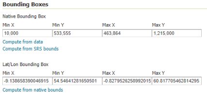
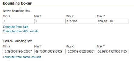
Bounding Box recommendations – Layer Config
Scotland
Min X = 010000
Min Y = 533000
Max X = 464000
Max Y = 1215000
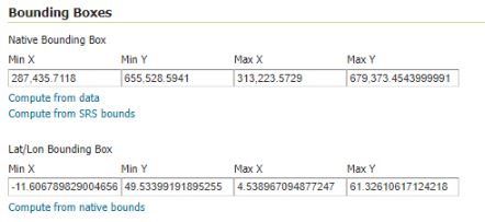
West Lothian
Min X = 287000
Min Y = 655000
Max X = 314000
Max Y = 678000
UK
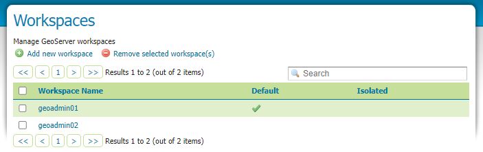
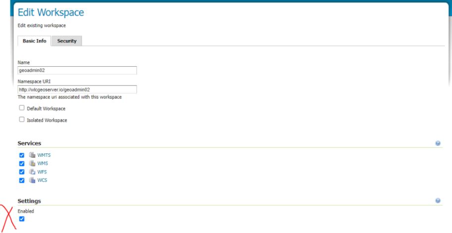
Workspace setup and visibility in WFS
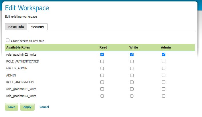
Workspaces can allow for editing and not editing of information although to date I seem to be struggling to isolate layers and workspaces to allow them to be edited or not edited. One thing that is important in our present system is to Enable the settings in the Basic info – without this the layers within the workspace were not showing up in the WFS
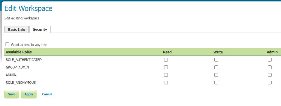
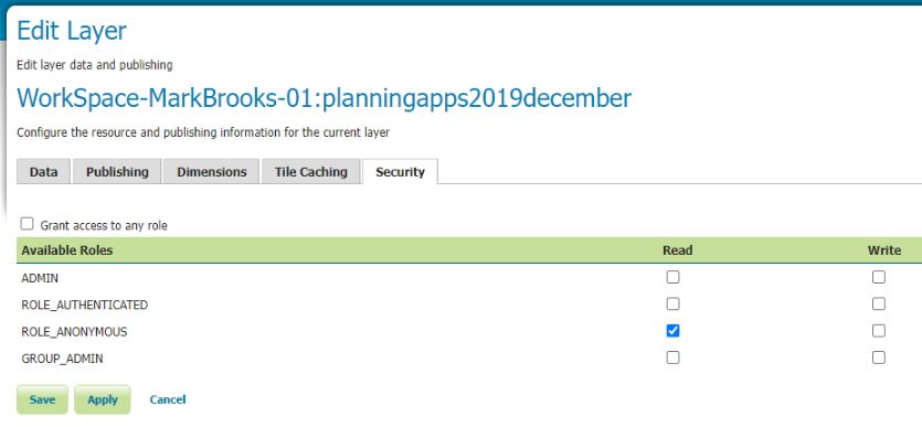
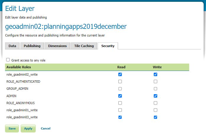
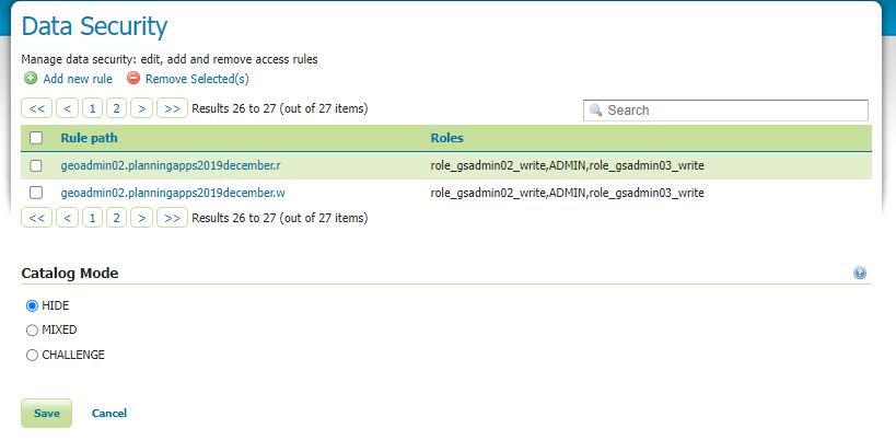
Restrictions on Layers : Important Note
Important – Workspace Security settings override Layer Security Settings
If you need to have different layer security settings within one Workspace you will need to turn off all Workspace security settings e.g see below.