Planning in the UK has for a long time suffered from a classic siloing of data by authority resulting in slow and varied analysis of information. Authorities relied on talented motivated individuals with particular interests and skills to develop bespoke solutions that assisted in the development of things like housing land audits , population forecasts , capital planning and local plan development which while often impressive individually struggled to transfer between authorities.
The continual improvement of digital tools has dramatically improved standardisation of the attributes of particular spatial data sets and database technology originally developed for accounting systems and flight control systems is starting to be applied to the amalgamation and analysis of planning related information. Within the UK different regions are progressing along this path at different rates. Scotland now has a body the Improvement Service who has a specific remit to collect spatial planning data which they do at something call the Spatial Data Hub.
The Spatial data hub at 08 January 2024 had 59 datasets listed at Scotland coverage level. Including
Planning application boundaries
School Catchment Areas
Housing Land Supply
Vacant and Derelict Land
Employment Land
The improvement service has been building these datasets for a number of years now however last year they expanded general access to much of the information and I have since been experimenting with it to see what can be achieved.
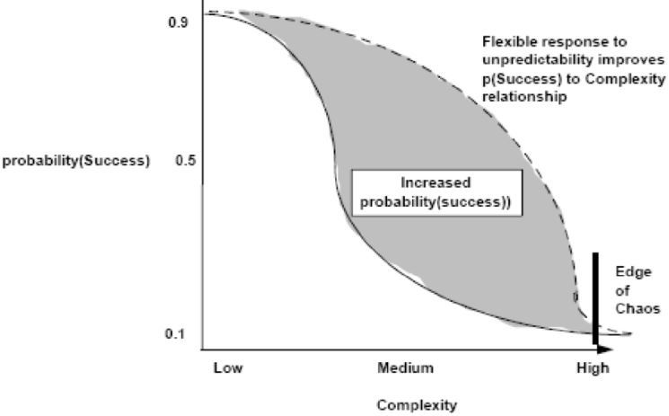
I don’t do that many strategic posts these days (compared with my first posts) but this is really a reminder to myself to always seek out the simplest solution especially when configuring systems and writing code. Less is generally always better. The above post was a DALL E production and the below graph is the simpler one which QED actually makes sense. I would suggest that the line moves to the right with improved education of staff / time / money and number of staff but eventually productivity dramatically drops with complexity no matter how much money , time or people.
As soon as you need to practically implement any information in Spatial Databases display of the information through a mapping front end becomes absolutely vital. Many database administrators are used to simply going into their favourite database editors and displaying the raw subsets of tables and queries. That works well for financial transactions and inventory tables were collapsing the attributes of objects into single digits is often valuable or possibly preferable to simple photos. When dealing with boundary information the complete opposite applies. Display of information as simple screens of matrix numbers is completely useless.
Additionally often boundaries make zero sense unless referenced to the land beneath them either through aerial photography or topographic maps.
In a previous time where I worked we actually commissioned a company to give us aerial photos of a local authority. This was not an insignificant amount of money and was probably only marginally reduced by the vendor having multiple channels of sale. Google and Microsoft are now very good in offering very good aerial and line interpretations for limited use to companies and individuals. This is absolutely great as it can be used as background either to confirm accuracy of other information or as data upon which to calculate further information (eg routing).
So how can an individual get up and started with some of these basemaps.
Sometime recently (I know not when exactly) QGIS changed its implementation of Open Street Maps through their desktop – rather than being an additional plugin Open Street Map provision is now included on install.
Here I am working with QGIS version 3.10
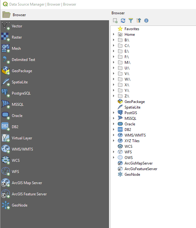
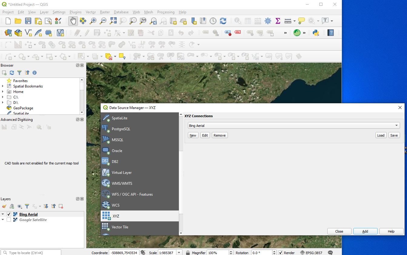
Now you should be presented with the Data Source Manager Dialog which looks like this
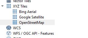
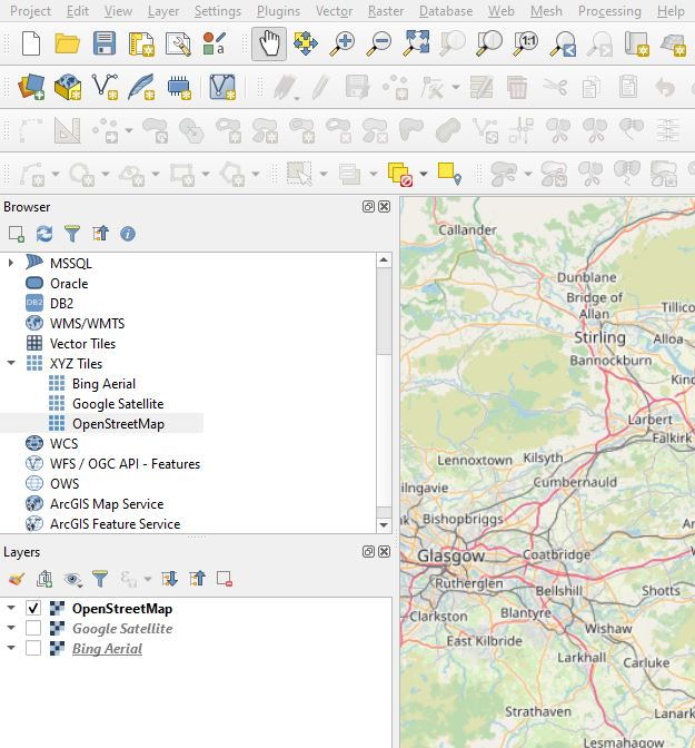
Now expand the XYZ Tiles
You can then double click on any one of the three and the WMS will be transferred into the layer panel
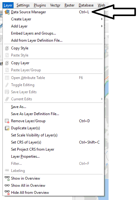
Layer > Data Source Manager > XYZ
Thank you to Google and Microsoft and OSM and QGIS for a great implementation.
A formula that can be used for calculating compound interest
A = P( 1 + (r/n) )^nt ; R = r * 100

Where:
A= Total Accrued Amount (Principal + Interest)
P = Principal Amount
R = Rate of Interest per year as a decimal
; r = R/100 so 4% is 4 and r would be 0.04
t = number of periods
n = compounding period
(^ indicates to the power of)

Note: Remember BODMAS when calculating with variables
Reasoning – this breaks interest down into individual compounding periods. For example, within a year when dealing with months, r would be divided by 12 if the source of interest is annual based. The individual periods are then compounded using the power over all the periods eg 24 periods for 2 years – see the examples below. NOTE the r/n is an empirical adjustment required because quoted interest rates from most sources are over a year (annual). Whenever obtaining interest rates from a source we must be careful with the r/n calculation as it may need to be ignored. If for some reason the period over which interest is defined in the source list is anything other than annually this r/n calculation may require alteration..
So for example if we want to calculate interest on £100,000 over a period of 4 years and 8 months based on an interest rate of 4.0% over the base of 0.5% over differing compound periods;
Compounded annually;
A = 100,000 ( 1 + (0.045/1) )^4.67 = £122,821.10
A = £122,821.10
Compounded Monthly;
A = 100,000 ( 1 + (0.045/12) )^56 = £123,319.40
A = £123,319.40
Compounded Daily
A = 100,000 ( 1 + (0.045/365) )^1704 = 123,376.30
A = £123,376.30
Please note : simplification this calculation leap years re-calculate if important
(^ indicates to the power of)
Methodology – How to calculate the Interest rate to be used
At the Bank of England the Monetary Policy Committee (MPC) made up of appointed members set the bank of England Base rate. When they do this it normally makes the national news. For example on the 3rd of August 2023 the Monetary Policy committee set the interest rate at 5.25%. This is the interest figure I use in the above compound interest rate when I need to calculate interest to be added by the council for holding money over a given period. But because for any given period it is unlikely that interest rates will have been uniform for the entire period it is necessary to either calculate one figure for the entire period or alternatively calculate the interest on the principle for each sub period and aggregate the figure for each of the periods. Below shows a method of calculating a single average daily interest rate for any period given changes to the rates.
So for example:
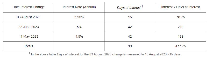
Calculate the interest rate to be used for a return of developer contributions received on the 11 May 2023 and required to be returned on the 18 August 2023 in the knowledge that the interest rate on the 11 May 2023 was 4.5% but was raised by the MPC to 5% on 22 June 2023 and then raised to 5.25% on the 03 August 2023. Develop a framework that can be used to calculate an applicable interest rate that can be used in the compounding interest rate calculation.
Average interest rate over this period is calculated as 477.75/99 or 4.825757%
This figure is consistent with the reporting by the Bank of England which changes rates on individual days rather than at the end of years or months. As such we should use the Compounding on a Daily basis to calculate the compounded interest to be returned as a result of holding this money for 99 days.
Normally, for developer contributions, additional interest will be calculated over periods of years rather than mere days but the above template can be used for any given time period. Additionally and importantly it calculates the total number of days which is also required for the compound interest rate calculation.
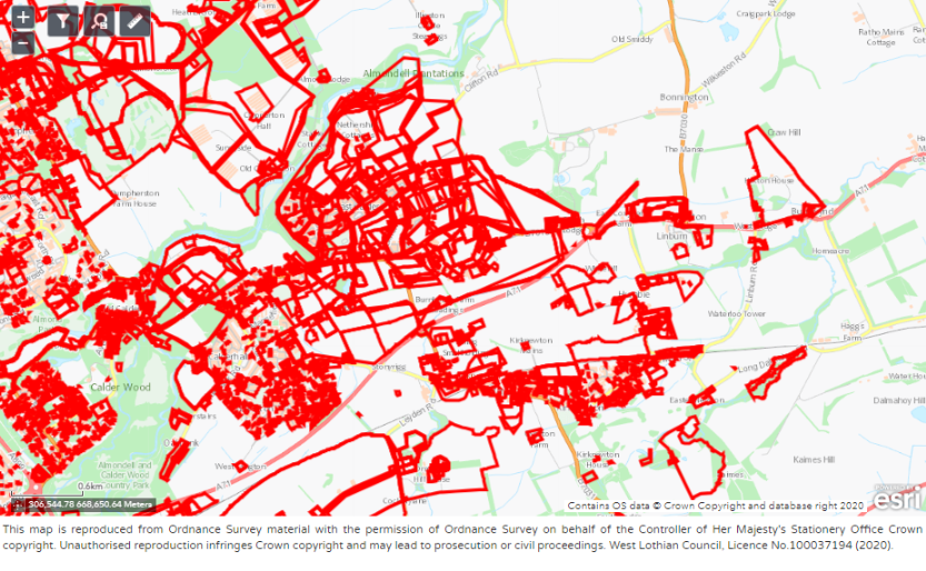
A significant number of authorities in the UK have the same software that allows members of the public viewing access to most of their recent planning application data. The last time I looked the software was in place for almost the whole of Scotland, Northern Ireland and close to 3/4 of authorities in England and Wales.
Part of this provision includes a public access web site that allows members of the public access to planning application details via a mapping screen. With practice this can be used to search and research planning application history. When first using the public website users tend to be defeated by the user interface.
Here’s a quick guide to assist in finding available planning applications relative to a particular site if you know its location on a map.
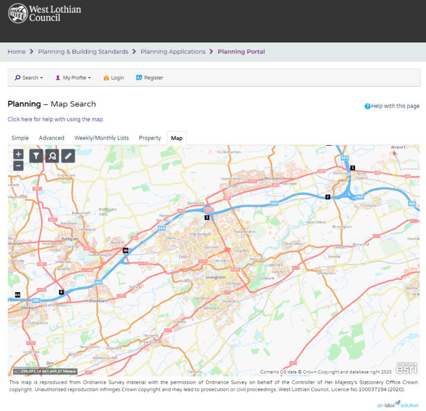
We will take West Lothian as an example. The UI slightly varies between councils but the principles are the same for a significant number of authorities
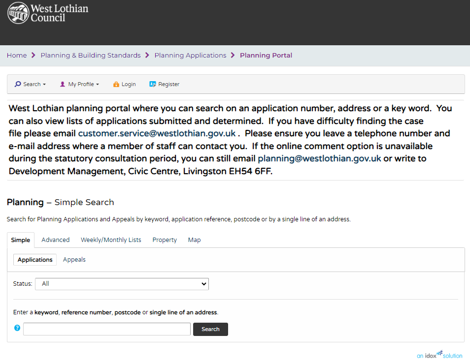
Firstly navigate to the Public Access Search screen of the authority that you are interested in.
You should be presented with the following screen.
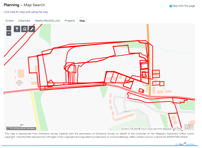
Two thirds of the way down on the right is a tab marked – Map – click this.
You should see something similar :-
Using your mouse navigate to the land parcel you are interested in determining the planning application history for.
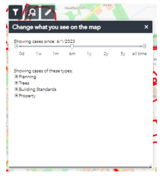
Next hit the filter ICON
Note on some authority sites this has been replaced by a drop down combination on the right.
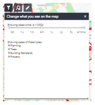
Hitting this icon on West Lothian site reveals a slider – initially it is set to 6 months for West Lothian
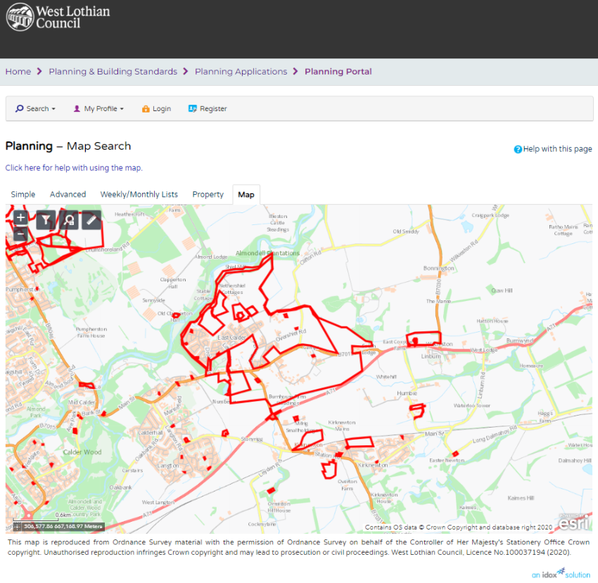
Chances are you will want to know all of the planning application history so move that slider all the way across to all time.
Now back on the map you should see many more boundaries representing many more planning applications.
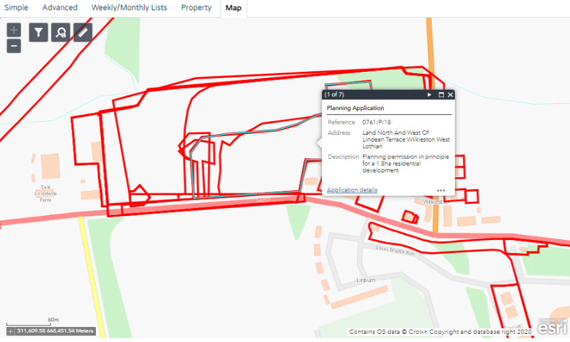
Users can now zoom in on the particular site they are interested in e.g. Wilkieston below
Now using the mouse you can click at the position you are interested in and the attributes of the planning application at the location you click will be revealed in a further dialog.
At this point you can note down the planning application references for further research or you can hit the link marked Application Details – here I click on the link related to 0761/P/18
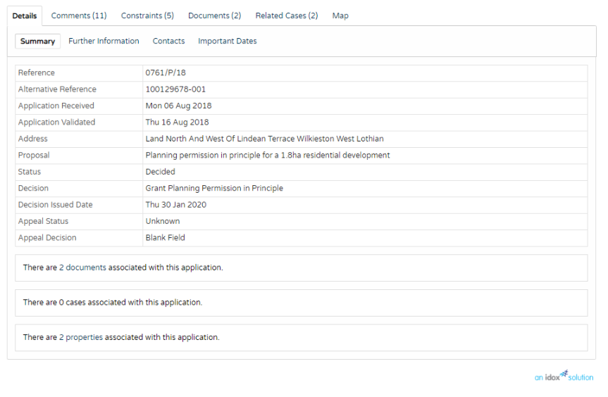
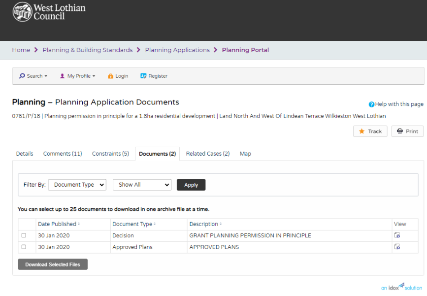
Which takes you to the Planning Application details page.
Want to see any available associated documents linked to the application.
Look to the text line beneath the table of attributes. The 2 documents is a link that takes you to available docs linked to the application. The number will be different according to the planning application.
Clicking on it brings up the Planning Application Documents screen where you should be able to download or view the documents.
Here’s a short guide I put together for myself to help me assess the value of enterprise systems that I may be looking for or designing myself. Not hard and fast and some points may not be relevant to every application but this should form a good basis from which to start. Generally a higher number is better than a lower number but within numbers items are more cumulative and of equal value.
1)Paper based = Everything from single sheets to formal Books of Accounts
2)Simple Digital = spreadsheet and other file based storage
3)Cloud based Simple Digital = spreadsheet and other file based storage – this can include file based blob storage
4.1)LAN relational database – normalised but otherwise fairly locked down
4.2)LAN relational database + easy import and export of data other than spatial
4.3)LAN relational database + report writer definable by users
4.4)LAN relational database + spatially enabled
5.1)Internet available relational database – normalised but otherwise fairly locked down
5.2)Internet available relational database + easy import and export of data other than spatial
5.3)Internet available relational database + report writer definable by users
5.4)Internet available relational database + spatially enabled (noted not all applications require a spatial aspect)
5.5)Internet available relational database + separate site available for public access view only
5.6)Internet available relations database + separate access to public access to edit and add information
Requirements
+ UPtime / reliability
+ SPEED – after reliability very important
+ Good master details forms (sounds easy but bootstrap is not great for this)
+ GOOD Search – the larger the system the more important the search options are in it. Look out for things like Automated Objective Index creation (case sensitive search is more of a hassle than a benefit a lot of the time – odd wild cards – or not being wild by default are problem areas)
Important Points
+ Portability can you up sticks and move it to a different cloud provider
+ Non – Proprietary (Can be a gotcha if its really obscure or has weird security, often linked to portability)
+ two factor authentication
+ Responsive Design (Not necessarily as important as you think in some applications see Github / Open Layers arguably don’t need it)
+ Dynamic saving – I really miss the fast dynamic saving environment of MS Access the save button isn’t quite the same
+ Built in CRM – I generally like them especially if data can go straight into correct files.. Increasingly I am designing systems with inbuilt CRM – I know this might not be to every organisations taste but it is jarring to go between systems and normalisation between systems is usually very sub optimal – plus you frequently come across proof of negative problems when data required for a specific task is not held appropriately.
+ Satellite application for customers to enter information (why not let your customers maintain their information can be great and can empower customers Fintech anyone?)
= All the bells and whistles
Spatially enabled internet available database with two factor authentication – report writer and easy import and export of spatial and attribute information with public access to edit and add information by customers (Possibly via satellite application).
This is a working example of how it would be possible to set up code that would automatically allocate for example housing sites to School Catchment areas. It could also be used to list constraints relevant to particular housing sites. This is more complicated in that it will indicate what percentage of the housing site is within which catchment areas and therefore allows for a single housing site being in multiple catchment areas. I am planning on coming back and expanding on this post. In this respect it represents a refinement of this Post
So we need two tables
t001asites which has a geometry field called geom
and another table which will be the catchments table called
t002bcatchments which has a geometry field called geom.
Both tables must have a serial primary key of pkid and both tables must be polygon data and the geom field MUST be defined as polygon and NOT multipolygon.
Air code is as follows.
1. Create table containing digitised polygons of housing sites.
2. Create table containing digitised polygons of catchments.
3. Measure the area of the housing sites and place that value in an area column within the housing sites table t001asites.
4. Split the housing sites by the catchment boundaries ensuing that each split polygon inherits the catchment it was split by.
5. Re-measure the areas of these split sites and add an area column to store the new calculations.
6. Divide figure obtained in 5. by figure obtained in 3 which will indicate the proportion of the housing site is in which catchment.
7. Perform a least remainder method on the individual sites grouped by their original housing sites to ensure the proportions sum to 1.
So to the code
BEGIN;
SET LOCAL check_function_bodies TO FALSE;
CREATE OR REPLACE FUNCTION part01catchjunctionmaker() returns void as $$
Alter table t001asites add column area integer;
$$ LANGUAGE SQL;
CREATE OR REPLACE FUNCTION part02catchjunctionmaker() returns void as $$
Update t001asites set area=ST_Area(geom);
$$ LANGUAGE SQL;
CREATE OR REPLACE FUNCTION part022catchjunctionmaker() RETURNS void AS $$
DROP TABLE IF EXISTS t200;
$$ LANGUAGE SQL;
CREATE OR REPLACE FUNCTION part03catchjunctionmaker() RETURNS void AS $$
CREATE TABLE t200 AS select a.pkid as t001pkid, b.pkid as t002pkid, a.area as t001area, ST_intersection(a.geom, b.geom) as geom FROM t001asites a, t002bcatchments b;
$$ LANGUAGE SQL;
CREATE OR REPLACE FUNCTION part04catchjunctionmaker() RETURNS void AS $$
ALTER TABLE t200 add column pkid serial primary key, add column area integer,add column proportion decimal (10,9);
$$ LANGUAGE SQL;
CREATE OR REPLACE FUNCTION part06catchjunctionmaker() RETURNS void AS $$
UPDATE t200 SET area=ST_Area(geom);
$$ LANGUAGE SQL;
CREATE OR REPLACE FUNCTION part07catchjunctionmaker() RETURNS void AS $$
DELETE from t200 where area=0 or null;
$$ LANGUAGE SQL;
CREATE OR REPLACE FUNCTION part08catchjunctionmaker() RETURNS void AS $$
UPDATE t200 SET proportion= cast(area as decimal)/cast(t001area as decimal) WHERE area > 0;
$$ LANGUAGE SQL;
CREATE OR REPLACE FUNCTION part088catchjunctionmaker() RETURNS void AS $$
DROP table IF EXISTS t201;
$$ LANGUAGE SQL;
CREATE OR REPLACE FUNCTION part09catchjunctionmaker() RETURNS void AS $$
Create table t201 as Select pkid,t001pkid,t002pkid, t001area, area, proportion, sum(proportion) OVER (PARTITION BY t001pkid ORDER BY t001pkid, proportion) as cum_proportion FROM t200 ORDER BY t001pkid, proportion;
$$ LANGUAGE SQL;
CREATE OR REPLACE FUNCTION part10catchjunctionmaker() RETURNS void AS $$
Alter table t201 add column value decimal (14,9),
Add column valuerounded integer,
Add column cumulvaluerounded integer,
Add column prevbaseline integer,
Add column roundproportion integer;
$$ LANGUAGE SQL;
CREATE OR REPLACE FUNCTION part11catchjunctionmaker() RETURNS void AS $$
UPDATE t201 set value = proportion * 100;
$$ LANGUAGE SQL;
CREATE OR REPLACE FUNCTION part12catchjunctionmaker() RETURNS void AS $$
UPDATE t201 set valuerounded = round(value,0);
$$ LANGUAGE SQL;
CREATE OR REPLACE FUNCTION part13catchjunctionmaker() RETURNS void AS $$
update t201 set cumulvaluerounded = round((cum_proportion*100),0);
$$ LANGUAGE SQL;
CREATE OR REPLACE FUNCTION part14catchjunctionmaker() RETURNS void AS $$
update t201 set cumulvaluerounded=100 where cumulvaluerounded = 101;
$$ LANGUAGE SQL;
CREATE OR REPLACE FUNCTION part15catchjunctionmaker() RETURNS void AS $$
update t201 set prevbaseline = round((cum_proportion - proportion)*100);
$$ LANGUAGE SQL;
CREATE OR REPLACE FUNCTION part16catchjunctionmaker() RETURNS void AS $$
update t201 set roundproportion = (cumulvaluerounded-prevbaseline);
$$ LANGUAGE SQL;
CREATE OR REPLACE FUNCTION part17catchjunctionmaker() RETURNS void AS $$
DELETE from t201 where roundproportion=0 or null;
$$ LANGUAGE SQL;
CREATE OR REPLACE FUNCTION part18catchjunctionmaker() RETURNS void AS $$
alter table t201 add column proppercent decimal(3,2);
$$ LANGUAGE SQL;
CREATE OR REPLACE FUNCTION part19catchjunctionmaker() RETURNS void AS $$
update t201 set proppercent = cast(roundproportion as decimal)/100;
$$ LANGUAGE SQL;
COMMIT;
and now a function to pull it all together;
CREATE OR REPLACE FUNCTION createcjt()
RETURNS TEXT AS
$BODY$
BEGIN
PERFORM part01catchjunctionmaker();
PERFORM part02catchjunctionmaker();
PERFORM part022catchjunctionmaker();
PERFORM part03catchjunctionmaker();
PERFORM part04catchjunctionmaker();
PERFORM part06catchjunctionmaker();
PERFORM part07catchjunctionmaker();
PERFORM part08catchjunctionmaker();
PERFORM part088catchjunctionmaker();
PERFORM part09catchjunctionmaker();
PERFORM part10catchjunctionmaker();
PERFORM part11catchjunctionmaker();
PERFORM part12catchjunctionmaker();
PERFORM part13catchjunctionmaker();
PERFORM part14catchjunctionmaker();
PERFORM part15catchjunctionmaker();
PERFORM part16catchjunctionmaker();
PERFORM part17catchjunctionmaker();
PERFORM part18catchjunctionmaker();
PERFORM part19catchjunctionmaker();
RETURN 'process end';
END;
$BODY$
LANGUAGE plpgsql;
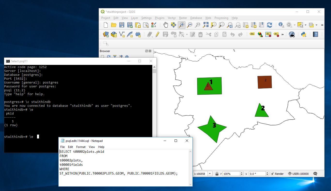
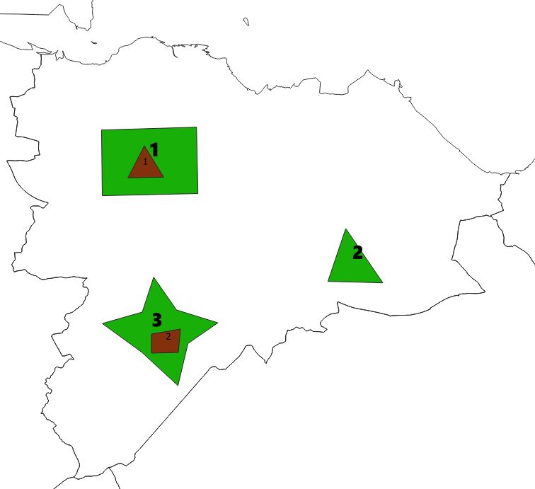
Now lets go to QGIS connect to the PostGIS instance add the tables and create some test data manually.
Here I have added fields in green with bold number labels and plots in brown with smaller number labelling. The numbers represent the pkid fields.
Now here I can quickly run a query to identify the plots that are in fields
SELECT t00002plots.pkid
FROM
t00002plots,
t00001fields
WHERE
ST_WITHIN(PUBLIC.T00002PLOTS.GEOM, PUBLIC.T00001FIELDS.GEOM);
And it correctly identifies that plot 1 is within the fields layer.
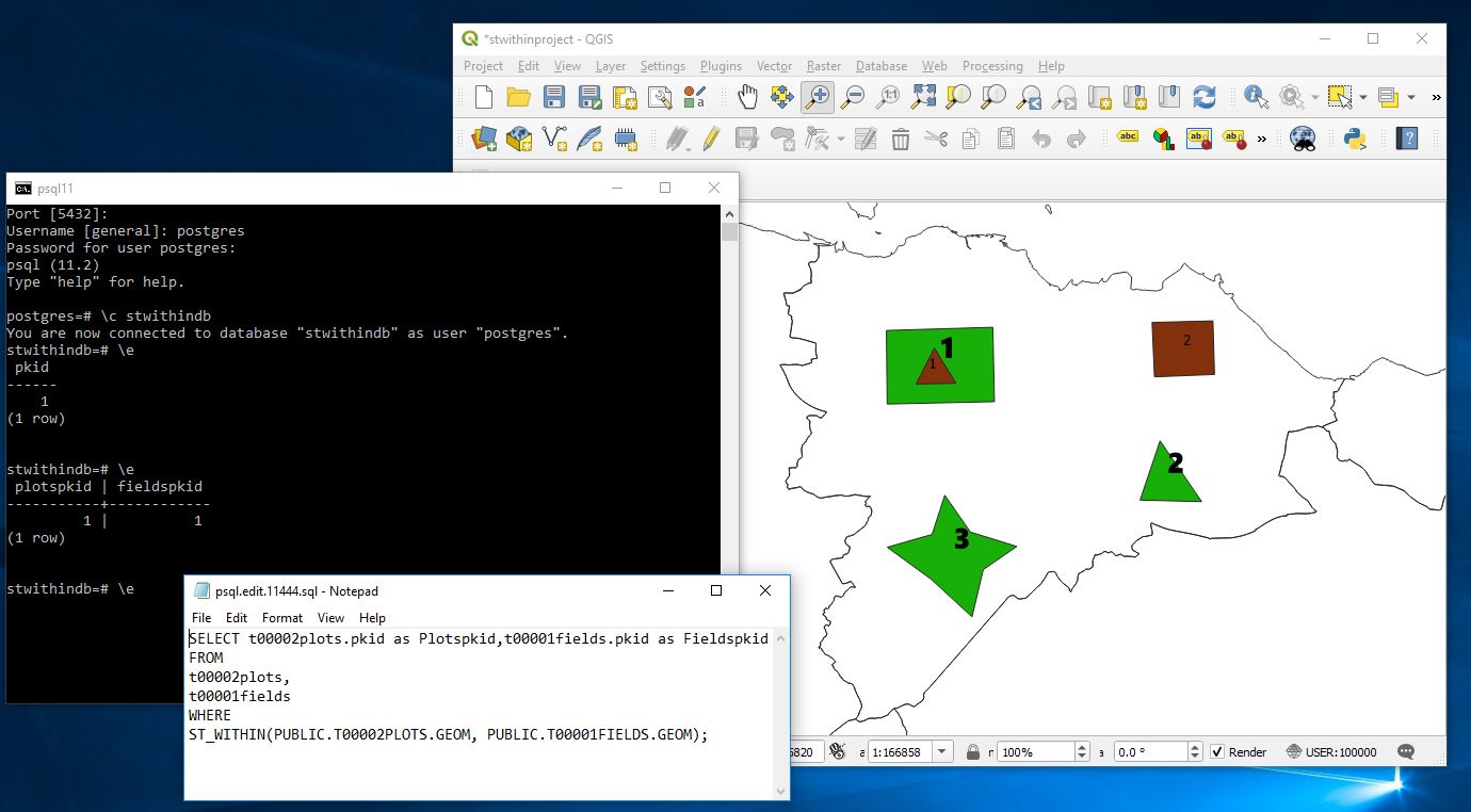
But what would be great in an application is to have some kind of junction table that individual master records could display their children on. For this we need a junction table that links between the field and plots table showing the pkids from each.
SELECT t00002plots.pkid as Plotspkid,t00001fields.pkid as Fieldspkid
FROM
t00002plots,
t00001fields
WHERE
ST_WITHIN(PUBLIC.T00002PLOTS.GEOM, PUBLIC.T00001FIELDS.GEOM);
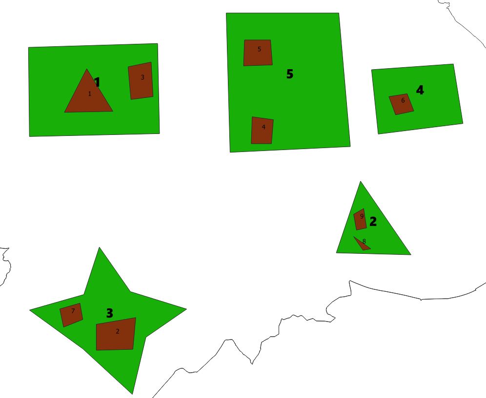
Now I will move plot 2 into field 3 and rerun the above.
The layer now looks like
and running the former query we get.
Now its possible to either create a junction table to hold this information..
eg
CREATE TABLE t00010fieldplotjunction AS
SELECT t00002plots.pkid as Plotspkid,t00001fields.pkid as Fieldspkid
FROM
t00002plots,
t00001fields
WHERE
ST_WITHIN(PUBLIC.T00002PLOTS.GEOM, PUBLIC.T00001FIELDS.GEOM);
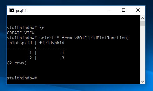
or we can create a view that will constantly calculate this everytime it is seen
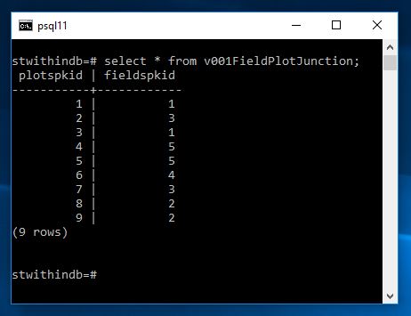
CREATE VIEW v001FieldPlotJunction AS
SELECT t00002plots.pkid as Plotspkid,t00001fields.pkid as Fieldspkid
FROM
t00002plots,
t00001fields
WHERE
ST_WITHIN(PUBLIC.T00002PLOTS.GEOM, PUBLIC.T00001FIELDS.GEOM);
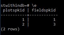
Now if I add a few more plots and fields and then pull up the view we shall see that everything has been adjusted
and running the view we now get
In some circumstances this calculation may be expensive so we may wish to run and create a junction table overnight other times we may be happy to do it fully dynamically. Of course in a front end you could query and filter such that only one record was compared against the fields plot at anytime. Very useful nonetheless.
In 2017 I was involved in an important work project to transfer all the records in a legacy system that was being deprecated by the vendor (IDOX Group) into another maintained system. We were in some ways fortunate because both systems had been designed by a single company (IDOX) and they were encouraging us to transfer. We had delayed transfer for several years already but were aware that we now had to move. The vendor did have some tools in place , had staff dedicated to such transfers and were offering favourable consultancy rates. The amount of data was not horrendous in computing terms but they were far far beyond the remit of the ability to cope with any sort of manual data correction and the system was an absolute core system upon which several departments completely depended. These were systems that all departments are in from the moment they start the work day to the end. Generally its unusual if they are down for more than 5 minutes in a month, all work pretty much stops when they stop and in no circumstances could they be down for more than a day without special dispensation and coordination to indicate to manage customer expectations.
The whole project was a success although it was challenging. Here is an outline of the steps we took. As ever order here is important in most of the steps. I had written something on this before but consider this to be a more accurate rundown see here
Step 1
Inform managers of all involved sections and ensure they are on board – identify and ring fence budget
Step 2
Appoint project manager on vendor and client side
draw together team to perform transformation.
Step 3
Draft time table creation of how long it will take putting in place planning for tutorials on systems and consultancy.
Step 4
Request managers to put forward staff on all sides willing to be involved
Step 5
Identify any omissions in knowledge and start to identify how this can be remedied. Kick off and complete acquisition of said staff.
Step 6
Meeting with lead staff to confirm buy in. Request buy in from staff including ring fencing of holidays etc.. to ensure key staff are available at required times.
Step 7
Set up test systems that all individuals have access to and ensure that the old and new systems can be viewed simultaneously by individuals. Ensure that the domain specialists can identify processes that will be mirrored from the old system to the new system
Step 8
Give DBAs or those that will be doing data transfer access to databases of source so that they can start thinking of how they can pull out information.
Step 9
Training for all individuals concerned in new systems.
Step 10
In new system start tasking individuals with how they are going to do the simple processes – eg register a record approve a record alter a record and get reports out. If possible allow new champions to start to define things like reports.
Step 11
Start making up any new lookup fields compared with old lookups and also start tasking individuals with creation of reports and letter that will need to be done.
Step 12
Start mapping the data from old system to new system – excel spreadsheets can be used for this that show the data going from the old system and what fields they are going to go into in the new system. Divide this task up between domain users – this step needs to be done after old and new systems are on domain users machines. As part of this the applications in question should expose if possible the table and field names of the source and target fields. With the systems we were involved in this was possible both for the old and new systems.
For each form on the two systems try to identify the below
Source table.field Target table.field
Also get them to map the lookup table values if direct transfer is not possible or if alias id are used in these lookups.
Step 13
Give both mapping documents to the ETL people to allow them to start writing the queries. It is unlikely that there will be a straight transfer across from table to table. While it would be expected that field and table names will be completely different it will be expected that table structure will in certain places be different in this respect it would be good to have a really nice schema diagram of both source and target.
Step 14
Allow data individuals to write scripts that can be run live against present initial system – if necessary doesn’t need to be live live could copy every night and then perform on 1 day old database backend – which is what we did. This means work can go on in old system and then at a touch of a button.
Encourage DBAs to be able to run these scripts every day to ensure that running them for go live is absolutely no issue. Our scripts only took about half an hour to run so this wasn’t an issue. I was personally involved in writing the SQL for those and I had systems in place to cross tab the amount coming into each new table so I could see new records and information from the old system trickling manually into the system and then being transferred.
Step 15
Test data input into new system
Step 16
Check test data input into new system with reference to domain users.
Step 17
Confirm go live date ensure staff available for issues
Step 18
Go live to production and start all new procedures ensure staff technical and domain key players on hand to make flexible solutions to things
Step 19
Project review on going maintenance and improvement of new system
Step 20
After suitable time turn off of old system if possible.
Objective here is to write a series of queries that can be used to measure the shortest distance between selected paired locations on a network such that the geometry of the routes can be calculated and displayed on a map.
For this particular tutorial you will need – QGIS 3 or higher and a version of Postgres I am using version 11.0 here (I have upgraded since my former posts). I believe this tutorial will work with previous versions but if you are following along now might be a good time to upgrade.
QGIS 3.4 or higher – needed as the Ordnance Survey road network geometry contains a z coordinate which will prevent the creation of the required geometry for measurement. QGIS 3 introduced the ability to save geometry excluding z coordinate. If you have a network without z coordinates you should not require this.
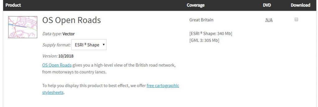
So let us first get the data. Here you tick the option in the top right hand corner – scroll to the bottom and submit your request after which you will be asked a few basic questions along with email address you wish the download to be sent to after a few minutes you should be sent the download link through your email – follow the instructions and you should be able to get the information
The information you are downloading is a block framework for the whole of the uk. When you unzip the download into a folder you will see multiple files. We will be using a section of the national dataset relating to Edinburgh – NT. Choose the block or selection that you are interested in. More blocks may take more time however.
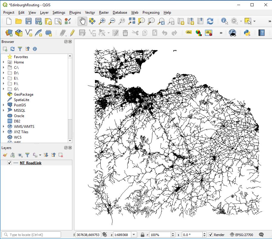
Open QGIS Create a new project : eg EdinburghRouting.qgz Load in your chosen network block : eg NT_RoadLink.shp
Select the layer you just loaded in : eg NT_RoadLink.shp
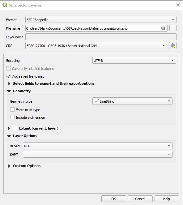
and navigate to the following in the menu settings Layer / Save As
Fill out the Save Vector Layer as … dialog box IMPORTANT – ensure within the Geometry section Geometry type is set to LineString Include z-dimension is unticked
Give the new file a name : eg ntosroutingnetwork.shp
Hit ok
Within the layer dialog of QGIS your new layer should appear you can now remove the for NT_RoadLink shape file from the project
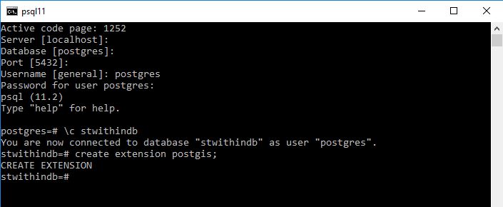
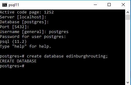
Next go to your version of PostgreSQL and using a superuser account create a new database : eg edinburghrouting
I would suggest you use lower casing as well
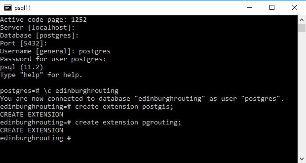
As a superuser ensure you add the postgis and pgrouting extensions.
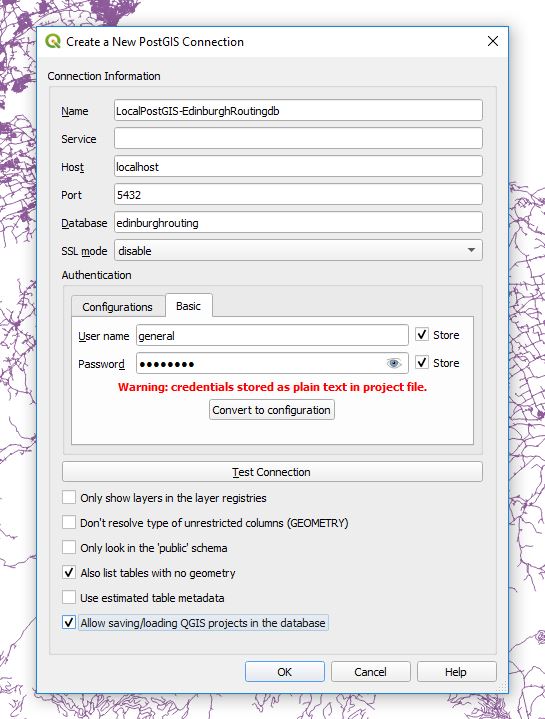
Next I set up the following connection between the QGIS project and PostgreSQL
Personal tastes may vary but I like like to select Also list tables with no geometry Allow saving/loading QGIS projects in the database
OK the selection and you should now have a connection to the new database you just created.
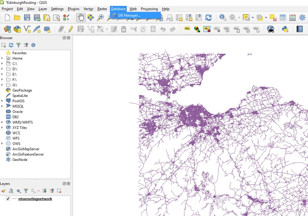
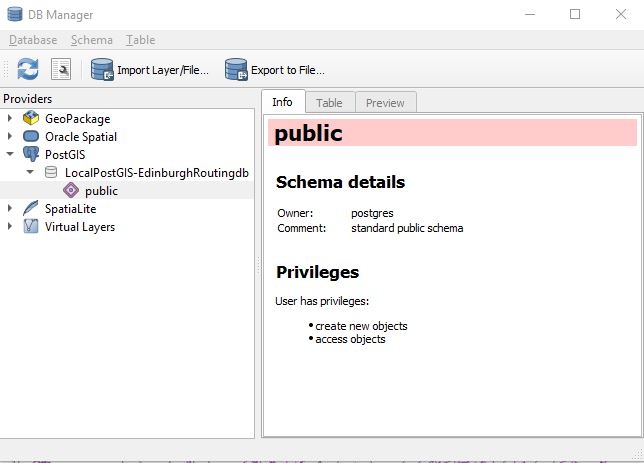
QGIS has an excellent dbmanager window which we will use to load our new shape file which excludes the z layer into the new database we created in PostgreSQL
Ensuring that you have a connection to your localpostgis database hit the
ImportLayerFile
Here I load the information into a new table t01roadnetwork
On pressing OK there will be delay after which if things go well you will receive the following message.
As ever it is good to check that things appear to be going well. Add the layer to your project and determine approximately whether import was successful.
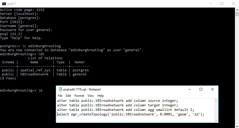
Next back in psql command line and in an editor we are going to run 4 queries The first 2 add columns that are required in the shortest distance algorithm we shall use, the third will allow anyone to write an aggregation function to see the total cost of the route and the last creates a topology for the road network.
alter table public.t01roadnetwork add column source integer;
alter table public.t01roadnetwork add column target integer;
alter table public.t01roadnetwork add column agg smallint default 1;
select pgr_createTopology('public.t01roadnetwork', 0.0001, 'geom', 'id');
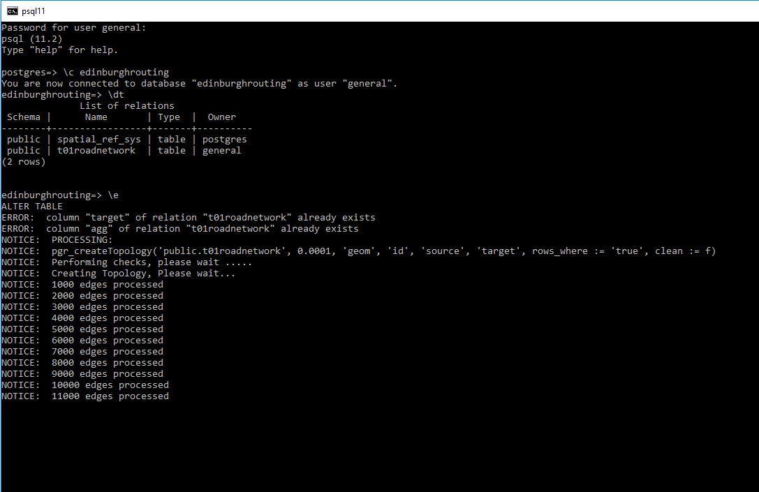
If things go correctly you should see the database engine start to create the topology and what I see is it gradually stepping through the creation process.
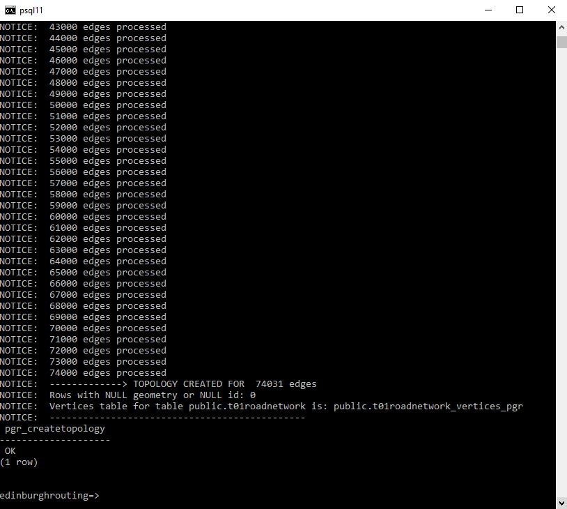
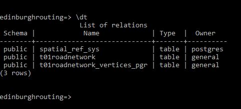
and on completion you should have something like the following:
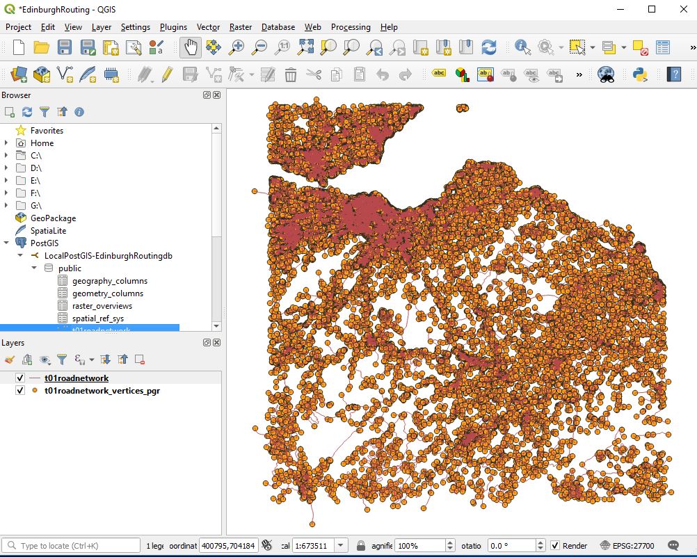
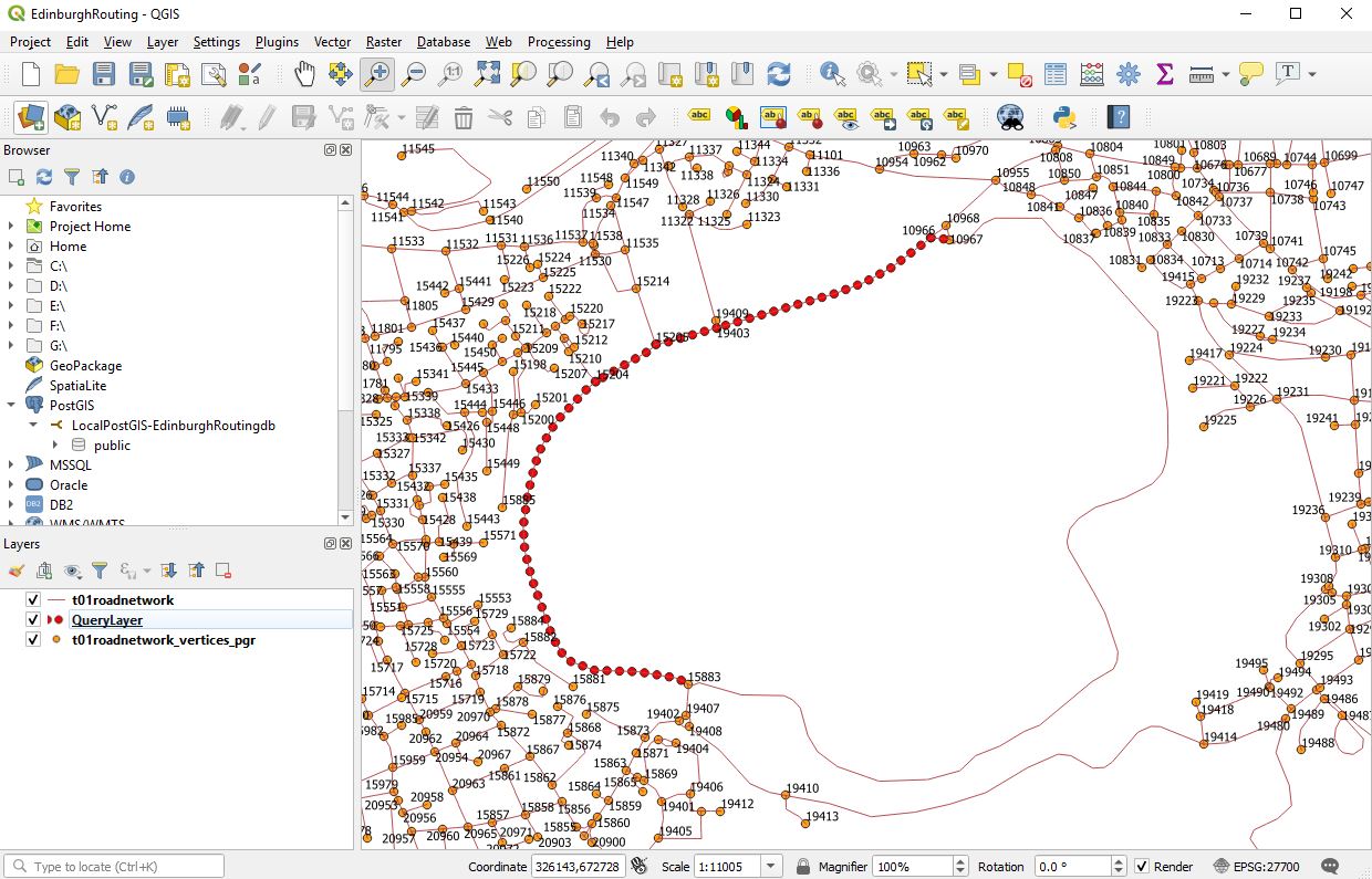
A new table has been added to the edinburghrouting database and next step is to display the network and its vertices. In QGIS.
In QGIS we should see something like
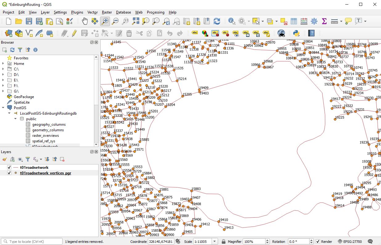
The next thing that I like to do is to label the nodes so that for quick identification.
And look to the t01roadnetwork table and see if the columns are clear and present.
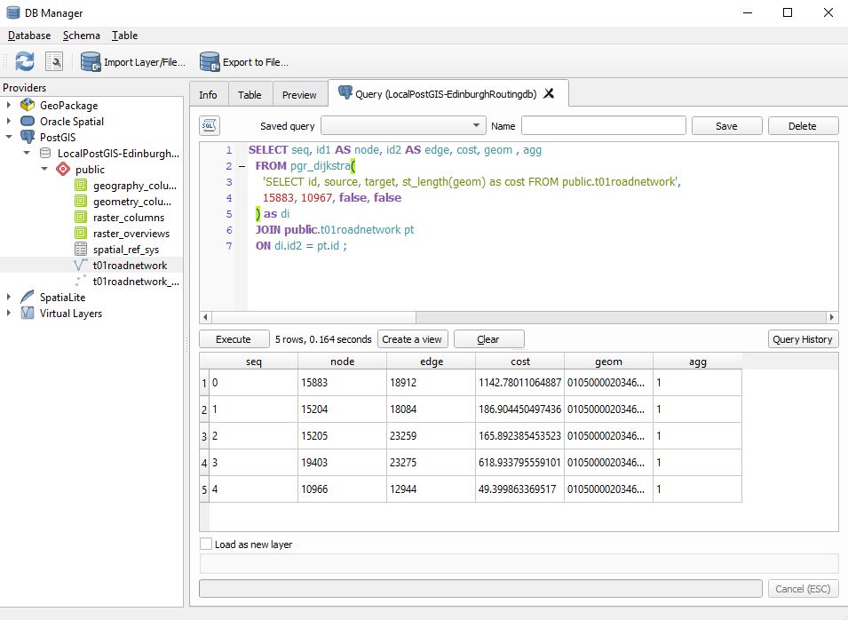
We are now ready to make a measurement. Here I choose the nodes 15883 and 10967
SELECT seq, id1 AS node, id2 AS edge, cost, geom , agg
  FROM pgr_dijkstra(
    'SELECT id, source, target, st_length(geom) as cost FROM public.t01roadnetwork',
    15883, 10967, false, false
  ) as di
  JOIN public.t01roadnetwork pt
  ON di.id2 = pt.id ;
Now we can load this as a new layer and then improve the symbology
Doing this we get.
It should be noted that the line you see is a collection of lines. In my next post I will go through and indicate how we can amalgamate that into a single line for storage in a table.
Congratulations if you have got this far you should be able to measure the shortest distance between any two points on a valid network by altering the numbers.
The following is a workflow that can be used to get a raster base map of anything into QGIS which you then reference to Open Street Map Layers ready for digitising against. This will be useful for approximate digitising of masterplans and approximate digitisation of housing completions.
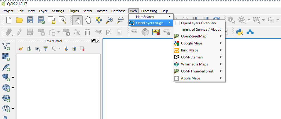
Firstly ensure you have dowloaded QGIS and added the following two plugins
OpenLayers Plugin
Georeferencer GDAL Plugin
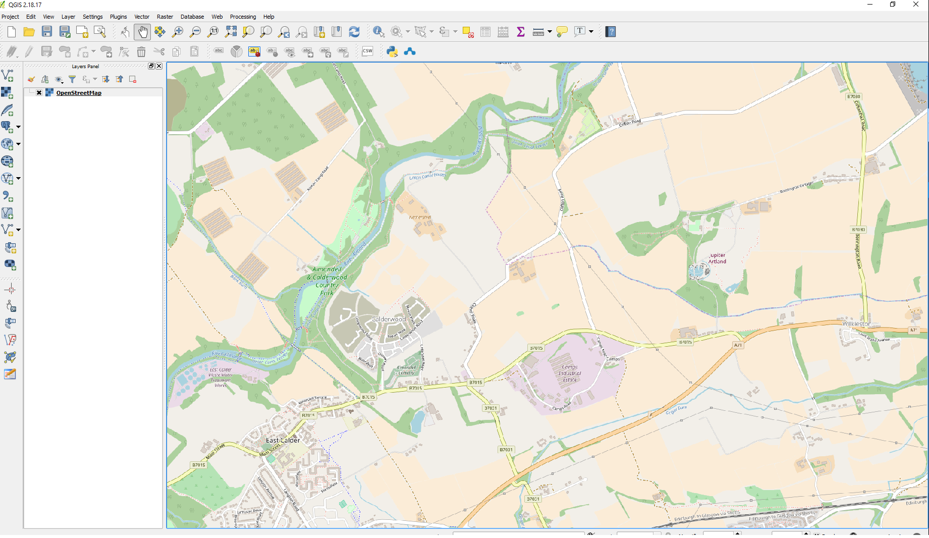
Opening QGIS now lets add the the Open Street Map Raster
From a blank project selection of Open Street Map should give you the following result
Now zoom to the approximate location where you wish to have a unique basemap. You will be referencing points on this map to points on your imported raster so you should zoom into a location to the extent that you can identify common locations between the two maps.
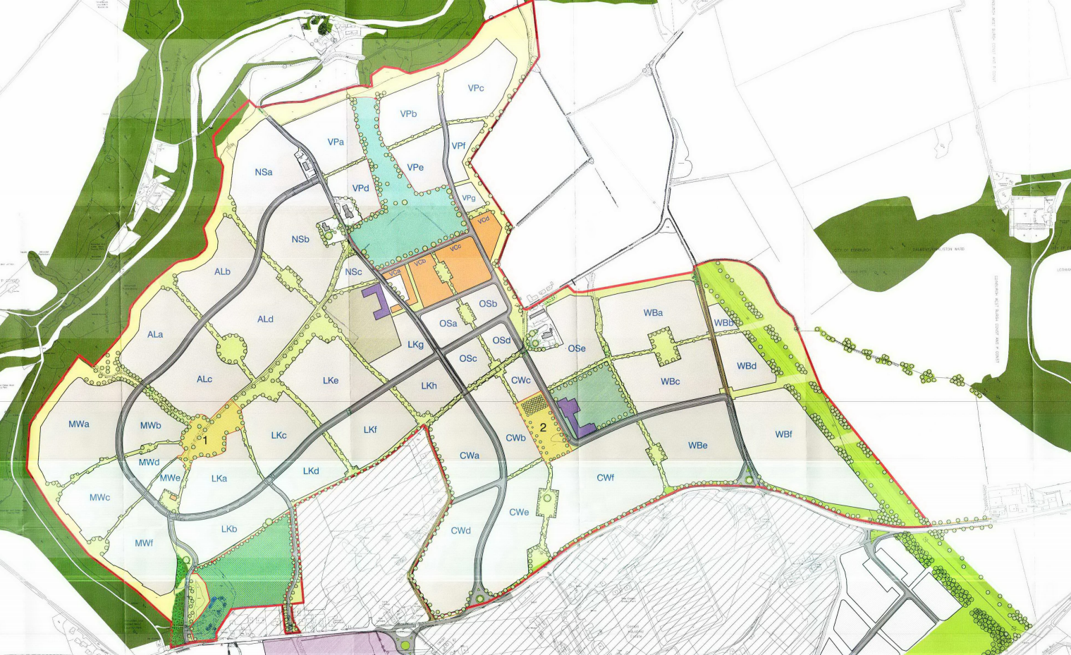
Identify the basemap you wish to have in your particular QGIS map here I choose freely available masterplan from Calderwood development in West Lothian from planning application 0524/P/09
Within the menus navigate to
Raster / Georeferencer /
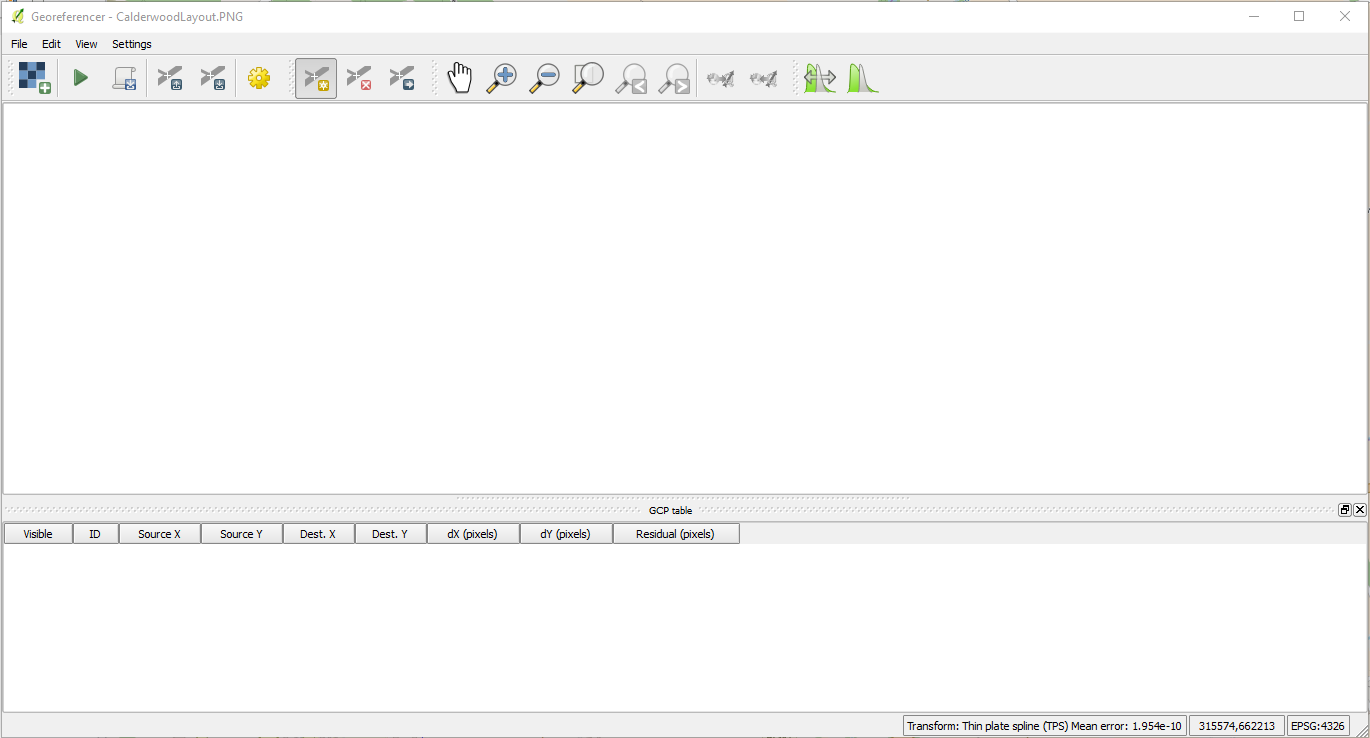
You should be presented with the following window.
Hit the add raster button in the top left
Select the basemap you wish to add to your project and ensure that the coordinate system that you choose is OSGB 1936 / British National Grid
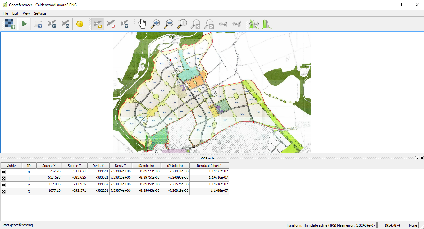
Next you want to add reference points to the basemap that will allow for you to put the basemap against it – This is done using the button marked
Next hit the settings button
You should now be presented with the Transformation parameters windows dialog as follows.
The dialog will remember old parameters if not ensure that you have the same selections (with your own selection of output raster location) as mine.
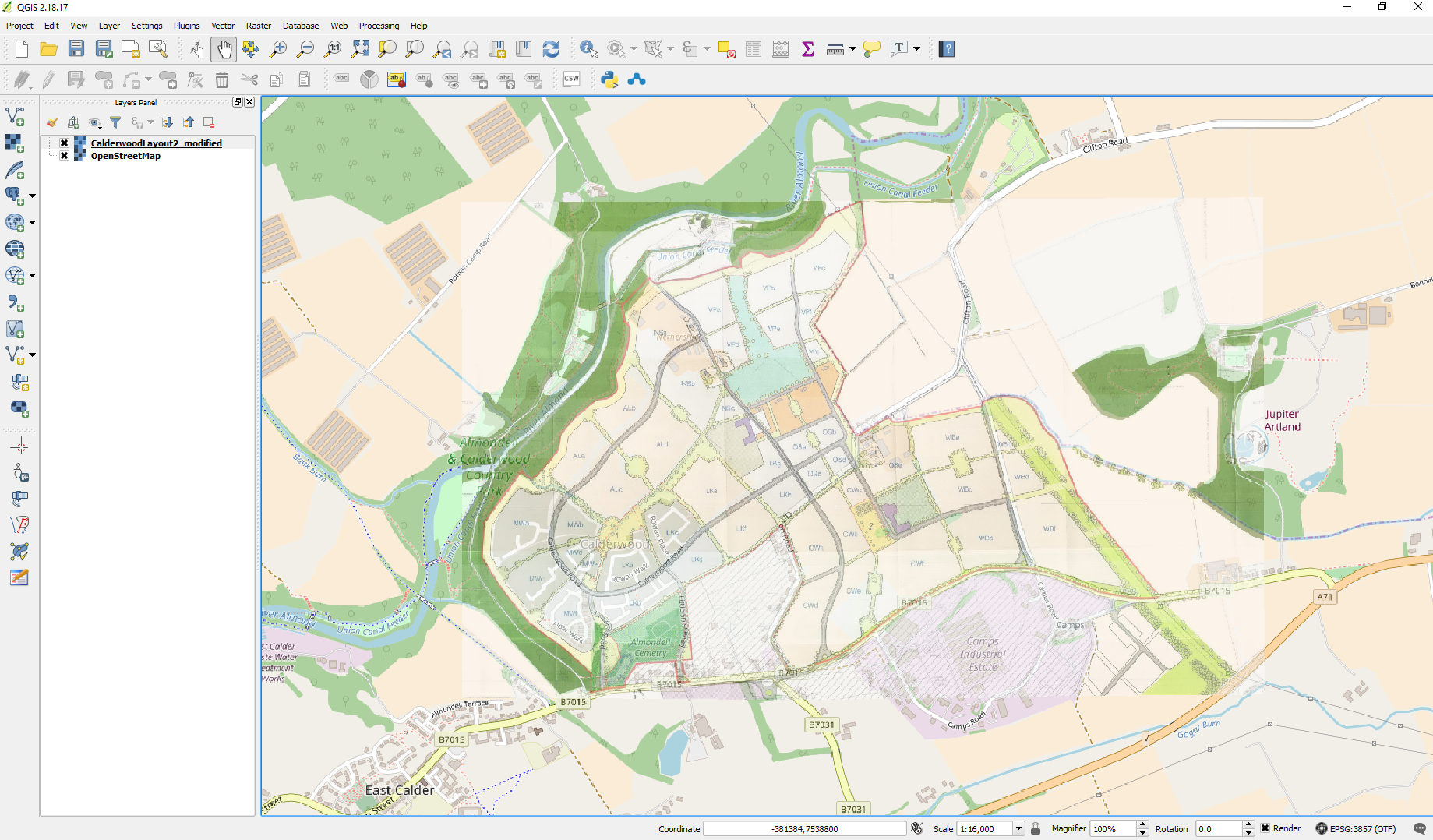
Now hit the play button the raster will be added to your map and the georeferencer will be reduced and moved to the bottom left of the corner where you will be open it and reduce it in size if you wish. You can now go in and alter the transparency so that it is possible to see both Open Street Map and your newly added raster
You should now be presented with something like the following – if there are red dots on the screen this is because you have not closed georeferencer down – simply open the window up again and hit file close.
If you are trying to design software that includes a Geographical element it is easier if you are working with data that makes some kind of sense.
The following are a list of sites where you can get good and consistent information on Local Authority Geographical Datasets within Scotland and in London. There has been an improvement in the quality and extent of information available but open data still remains patchy. Fortunately some datasets are available. The interesting thing about this data is that although it is rich it is largely unstructured and without relationships. Fortunately if there are geographical attributes then these can be used to spatialiy analyse the information and create relationships from which you can start to construct better systems.
I understand why the data is patchy. To really publish well it is a necessity to get your systems working well so that the export (and publication) of data can be at least semi-automated. Without this it is simply too onerous for staff to repeatedly perform Extraction Transformation and Load procedures on ever larger numbers of datasets. Taking a step back however therein may lie the benefit. The quicker they can learn to cleanly optimise and export and hopefully automate these procedures the more likely they are to have their systems working properly and importantly the more investigation and experimentation they can put into linking their datasets. The skills to link these datasets constantly to a web data portal being similar to the skills required to link between systems.
It might be expected therefore that better availability of open data is reflective of better internal systems.
Here is the information that I was able to identify through Google Searches at February 2018.
Many roles within organisations now require good project management skills especially when it comes to implementing new IT systems and applications. But are there things that can be put in place at the beginning to improve your chance of success. I would say yes and if I am involved in a project my personal guidelines are as follows;
Step 1 : Get Stuck In
The benefit of computers is that manipulated electrons are essentially free and immortal. Try to rearrange a few. If you aren’t getting anywhere wipe them and then re-arrange them some more. Even if you are not successful you are successful in knowing that one particular arrangement cannot be achieved. You are creating a machine just like children do with Lego or engineers create with bricks and mortar except your bricks can immediately be removed and copied infinitely and each additional brick often costs nothing. In most organisations you will quickly come up against configuration and security problems. Configuration and security problems come out of nowhere often and can be project killers best to know about them up front.
Step 2 : Know your Technology
If you don’t know it at the beginning you better hope you know it at the end – go to step 1 if you are struggling with step 2 – That’s recursion for you.
Step 3 : Increment often , test constantly and try to keep focused
Set short deadlines and try to regularly meet with colleagues or clients to show progress – can be frustrating if colleagues or clients start going off on tangents especially in meetings so try to keep focused on the remit.
Step 4 : Know the Process
To date I haven’t been asked to design any systems that I have had particular difficulty in understanding the process. Undoubtedly I think this would be different if I was trying to create an application for geology exploration or for instance mapping or maybe translation. The mathematics behind those kind of applications are complicated. Most business processes tend to be remarkably simple and the simple act of normalizing the data is usually enough for me to get to grips on how the system will be used.
Step 5 : Build in redundancy
Properly normalize your data build in extra fields if you want even if they are not used – for example collecting information on individuals I always add a field for date of birth even if its not spec’d invariably someone comes along and says actually it would be useful to know what age our customers are.
Step 6 : Have privileges
There’s nothing that will slow down a project quicker if you have to hand over responsibility of tasks to uninterested individuals who are not part of the project team. Better to have those people in the team and make sure they are on board with the importance of following through with the project.