
Once you have your data in an Enterprise Grade database sharing that information becomes important. Some vendors, in particular Digital mapping SAAS vendors want you to transfer your data into their clouds but for a lot of authorities that is categorically impossible for large segments of their data. For example about 3/4 of UK planning authorities run on software built by a company called IDOX Group plc which holds its data in Oracle this cannot be moved. For Geographical data here’s where Geoserver comes in.
From the website
GeoServer is an open source server for sharing geospatial data.
Designed for interoperability, it publishes data from any major spatial data source using open standards.
GeoServer implements industry standard OGC protocols such as Web Feature Service (WFS), Web Map Service (WMS), and Web Coverage Service (WCS). Additional formats and publication options are available as extensions including Web Processing Service (WPS), and Web Map Tile Service (WMTS).
Another way of putting it Geoserver allows programs that display and manipulate geographic information to display and edit that data while keeping it safe and secure and located in enterprise databases. It can connect to SQL Server / Postgresql and I am told Oracle which are the main relational databases used by Local authorities today so once setup and configured it could be used to compare and contrast information in one location from variable datastores. Datastores that for historical reasons cannot be moved. Here I concentrate on SQL Server because we have a particular issue with new systems needing to connect to SQL Server but it would be great if we could get it working with Oracle as well.
The following are my notes on installation and configuration of Geoserver on Windows linking to SQL Server and in this case a remote(not on the same computer) SQL Azure instance I believe any remote SQL Server instance would be similar. This post is a detailed explanation of the installation of Geoserver locally on a laptop but I believe installation would be exactly the same on a Windows Server machine albeit additional steps would be required to publish to the web either internally or externally.
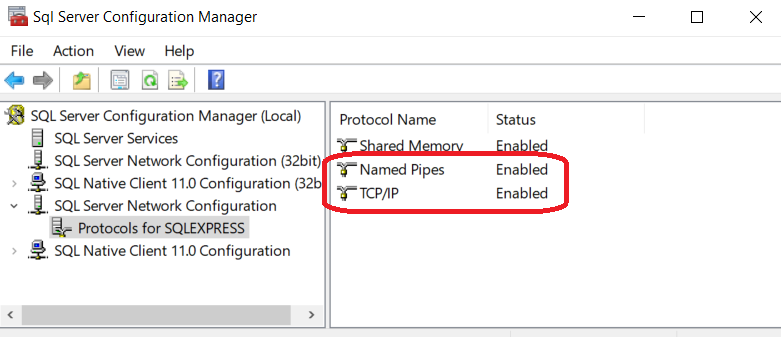
Its all configuration so remember your host names / IP numbers / ports / usernames / passwords / database, table and column names
To start this tutorial please ensure the following resources are available;
–
WorkFlow Synopsis Overview
1)Download and install Java runtime engine (as above importantly here I use 11)
2)Download and install Geoserver (2.24.1 in this case)
3)Test that the Geoserver Admin dashboard is up and working
4)Download and configure Geoserver Extension for SQL Server library (SQL Azure example)
5)Good idea to setup a login specifically to your SQL Azure instance with least privilege – Your SQL Server instance with geodatabases may already have suitable logins. So steps 5 and 6 can be skipped
6)Good idea to create an example table with Geodatabase in SQL Azure – will be used as a test connection table – NOTE if you already have a SQL Server with geodatabases you could use that instead.
7)White list IP within the SQL Azure instance firewall rules to Geoserver computer
8)Opening Geoserver and setting the ‘Store’ to reference your SQL Azure database using the login setup in step 5.
9)Adding a new layer from the Store made in point 8 and seeing if you can Preview the layer – Ideally you should have a table that has some features in it. Setting the WMS and WFS up in Geoserver with sufficient rights to allow editing (if WFS setup)
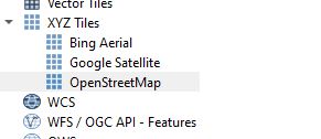
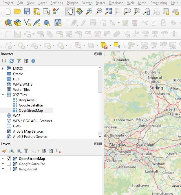
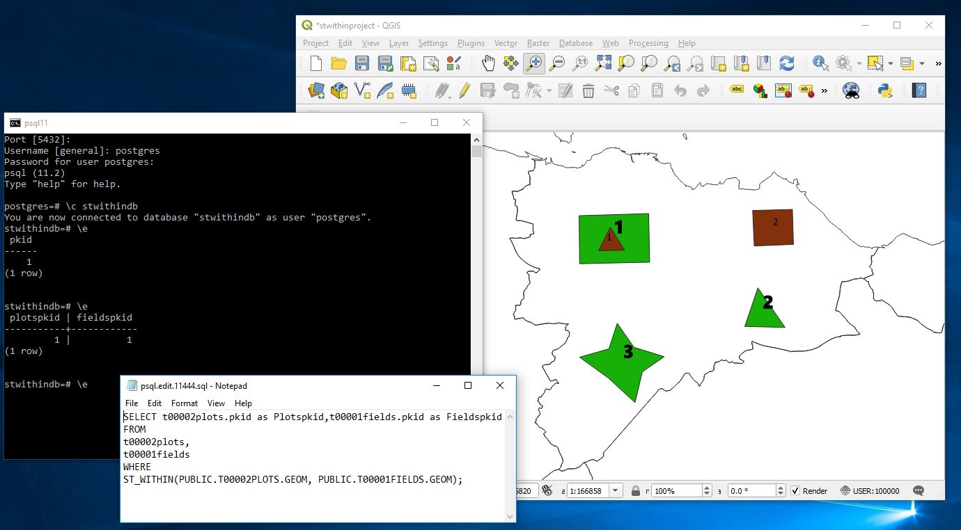
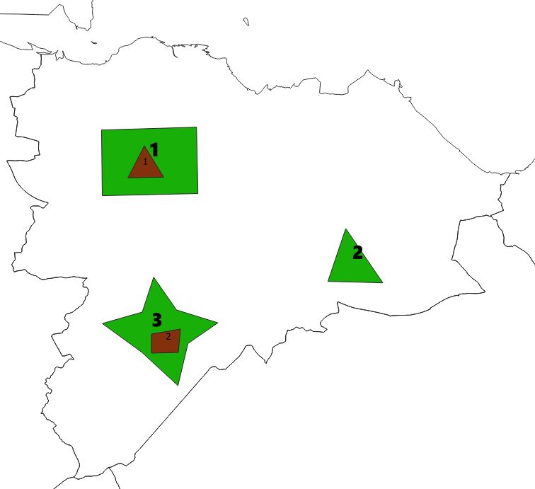
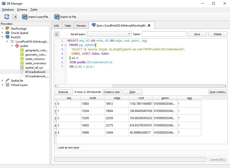
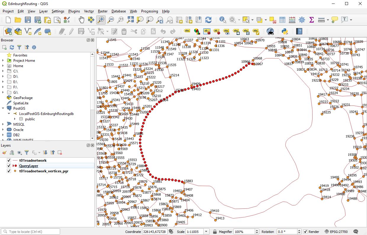
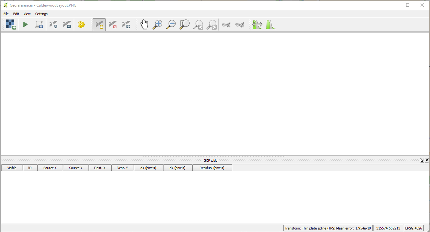
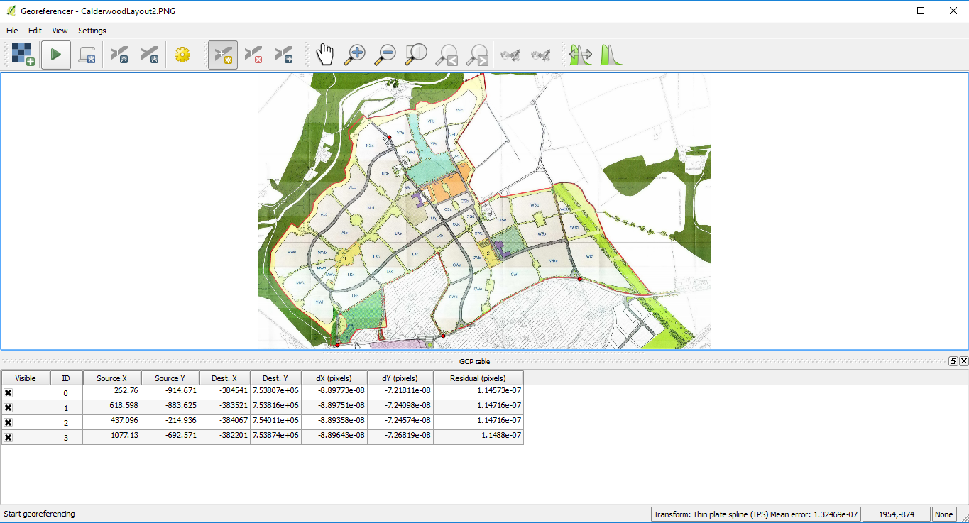
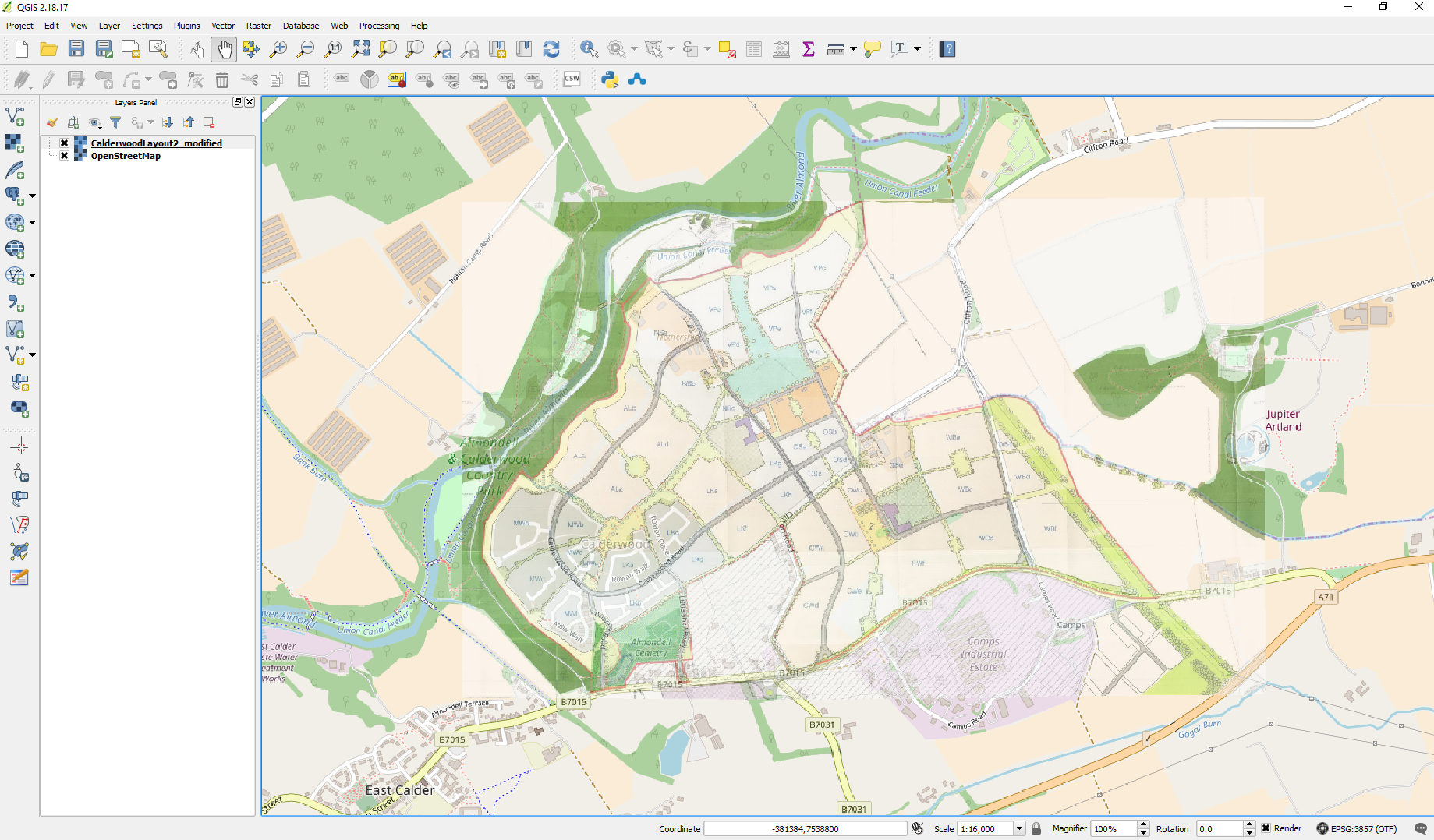
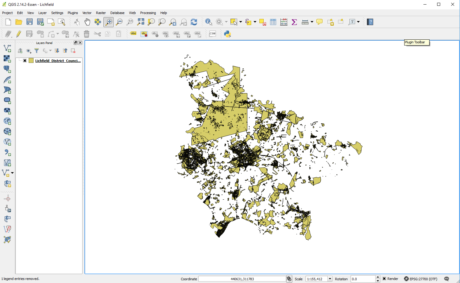
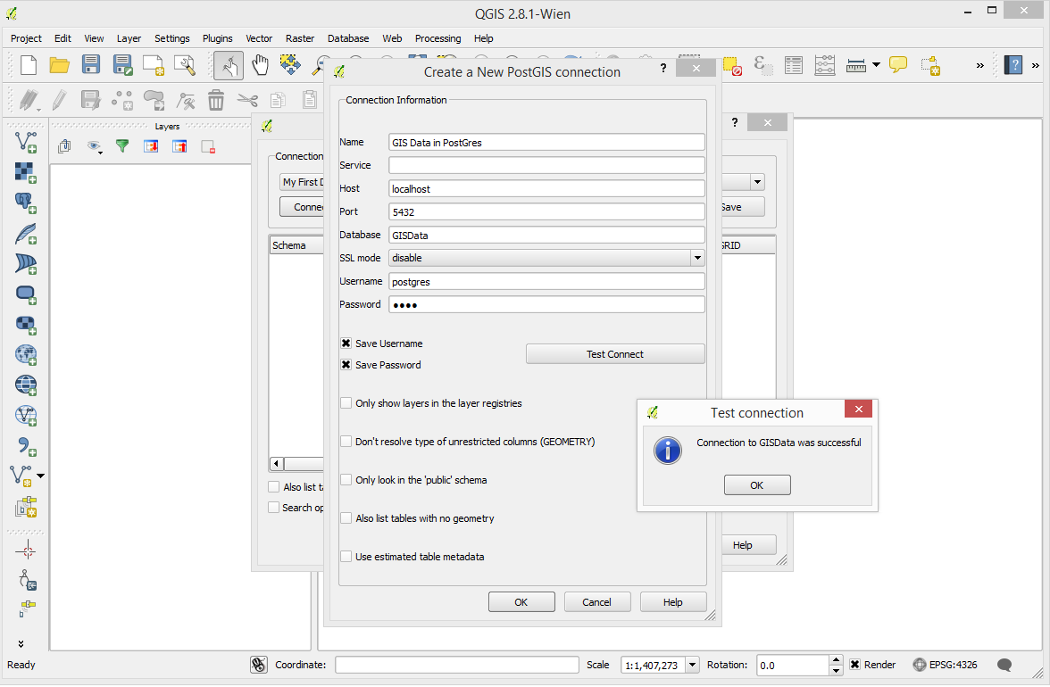
10)I don’t explain it in my post below but the next step would be to test in QGIS to see if you can setup a project in QGIS which can pull from Geoserver against a basemap and you check that the Polygons are actually where you want them to be.
Workflow Detailed
1)Download the install Java Runtime via JDK
There are some complications here
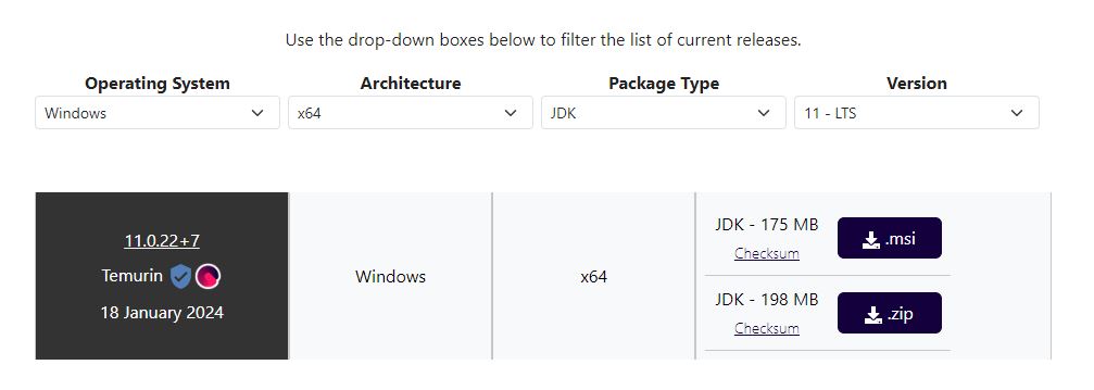
Initially I tried to use the Java Runtime engine 17 and went through the complete Geoserver installation but on testing I was getting a Java error when trying to view layers. After a short google I came across a stack overflow thread that indicated that geoserver support for JDE 17 was experimental and I should use Java Runtime engine 11. Deinstallation of 17 and installation of 11 solved this.
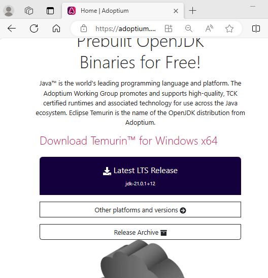
Additionally there is the issue of where you obtain the Java Runtime installation from – there is the Adoptium location and then there is Oracle location. Oracle are making moves to charge for use of their Java Runtime engine so it is important that you use Adoptium resource to reduce costs.
Later I will list the url to the JDK download for Java Runtime engine but it is important to realise that Adoptium is a safe source, well supported and noted as open source.
https://adoptium.net/en-GB/members/
so
Google Search for Adoptium
https://adoptium.net/en-GB/
Navigate to other platforms and versions and target windows 64 bit JDK and 11 LTS version and download the .msi.
After a short delay you will be shown the msi which will be in your downloads folder
Double click on it to install.
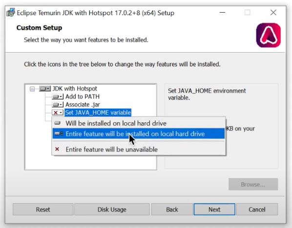
Now the only thing that is tricky here is to setup the java home directory as follows
Video Installing Adoptium JDK on Windows
In particular note this section
2) Download and install Geoserver
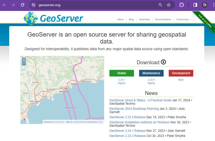
Go to the official Geoserver web page and follow the links to download the windows installer
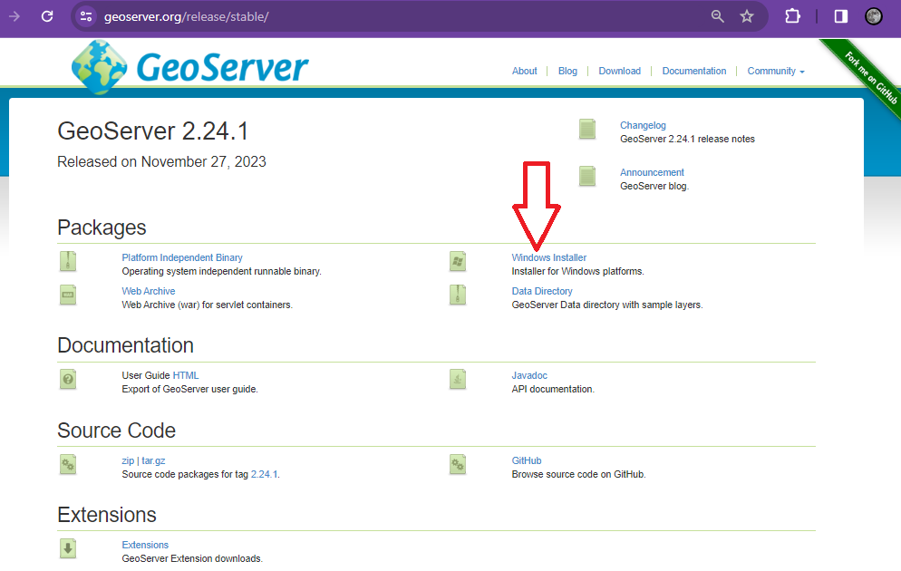
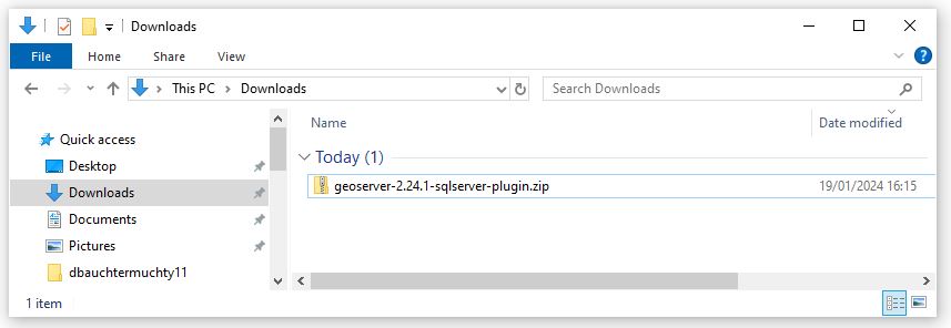
Here I use the windows version of Geoserver version 2.41.1 obtained January 2024 from the following url
Geoserver Official Website
See download button and then go to Windows Installer
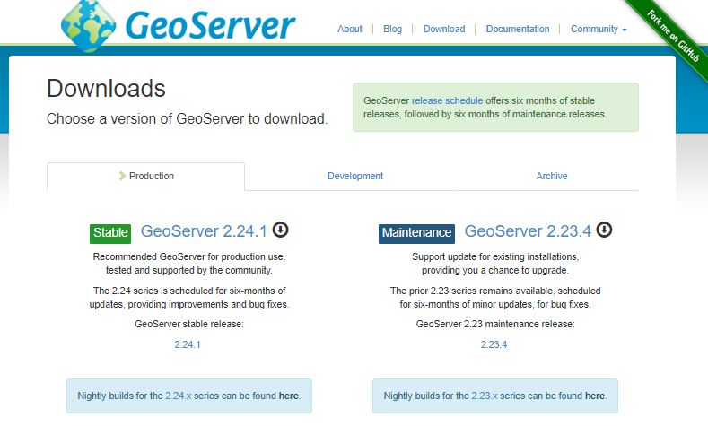
I chose the left option and then I chose the Windows Installer option
This will download Geoserver-2.24.1-winsetup.exe to your download directory and you can then start the geoserver installation process
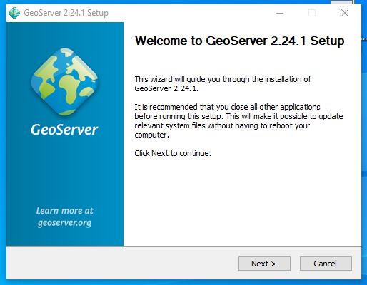
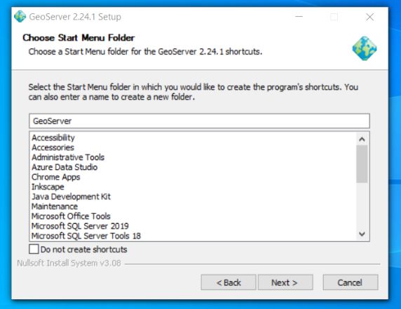
Next open up the executable and follow the instructions
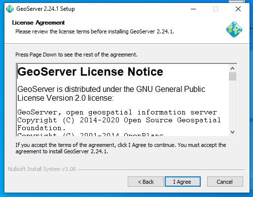
Next agree the licence
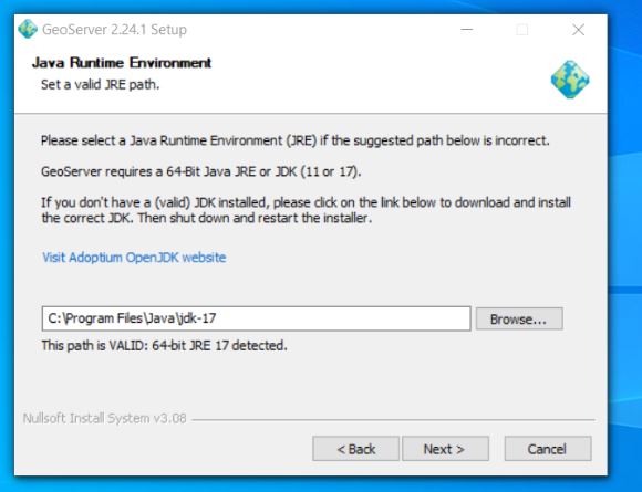
Next we reference the java library installed in the previous step – if you have set the java_home variable correctly it should automatically find JRE 11 for you and it will place it within the path reference below. I don’t have a screenshot of the JRE 11 reference here as on my first installation I referenced the Oracle 17 JRE – (note I went back de-installed geoserver installed JRE 11 and then reinstalled geoserver to counter the proprietary Oracle runtime library and importantly to fix the issue that I was facing of geoserver not being compatible with JRE 17
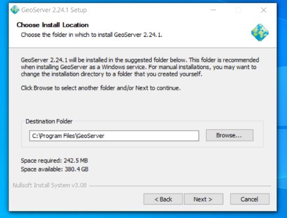
The rest of the install from here is standard for a windows install
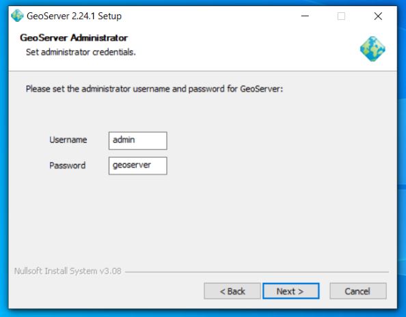
Next setup the default admin password – defaults are admin / geoserver
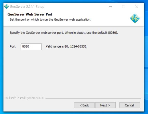
Set up port geoserver runs on – default is 8080
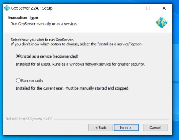
Next choose the execution type I like to install geoserver as a service
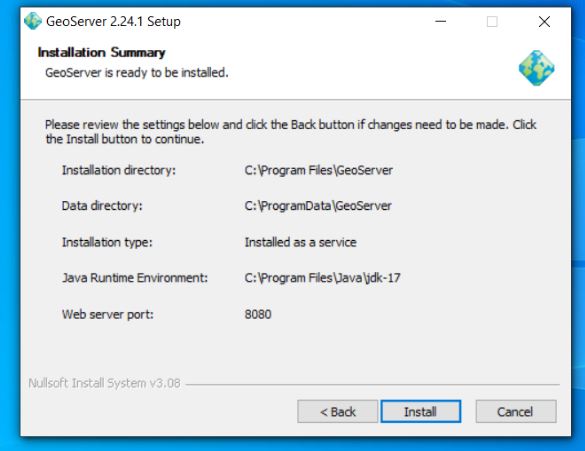
Confirm your preferences and then trigger install
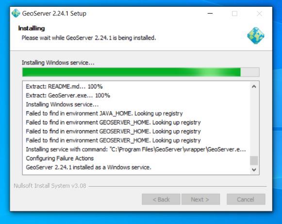
Now you should see geoserver on your local machine as a service which you will need to ensure is running to access properly
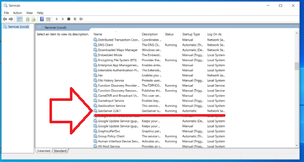
3) Test that Geoserver Admin dashboard is up and working at least locally
If you have used the same settings as me open a browser and navigate to the following url
https://localhost:8080/geoserver/web
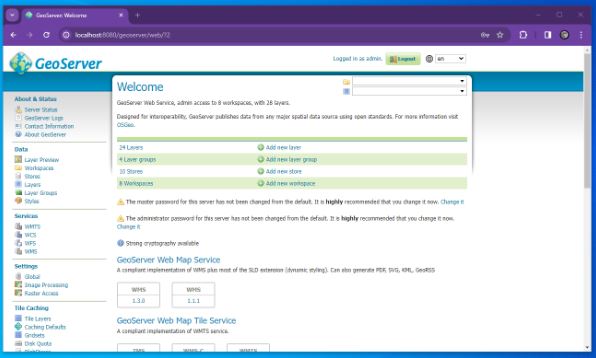
Login with the username and password which is usually admin / geoserver
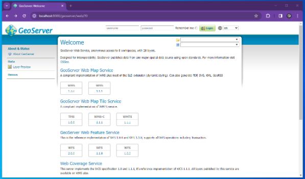
At which point you should see something similar to the following
4) Download and configure Geoserver Extension for SQL Server
At install Geoserver comes with the ability to connect to Postgres but NOT SQL Server so we must install/configure plugin extension to enable Geoserver SQL Server connections.
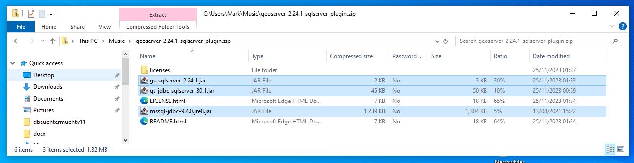
Here we go back to the geoserver.org website and go to download but this time instead of choosing the windows installer we look to the Extensions section and choose SQL Server
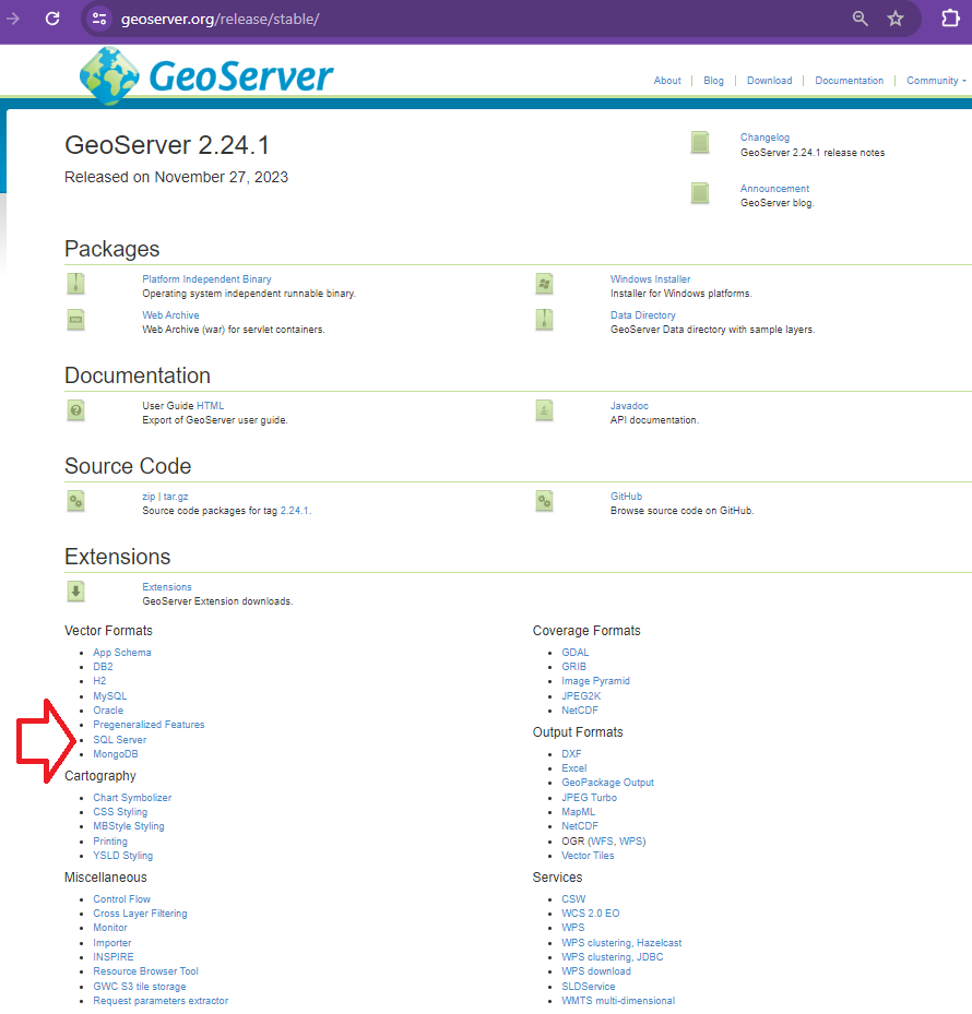
This should download geoserver-sqlserver extension plugin
Next copy all files with the jar suffix into the following directory
C/program files/GeoServer/webapps/geoserver/WEb-Inf/Lib
Next restart the geoserver and go back to the local host and sign in
http://localhost:8080/geoserver/web/?0
We are now very close to linking to SQL Server prior to that we must whitelist our geoserver so that your SQL Server instances will accept connections from your geoserver. Steps 5 and 6 are more about creating a user and ensuring you have a geodatabase with a georeferenced table skip to 7 if you want to read about white listing in SQL Azure or you have an alternative database that you could use with requirements already set up.
5) Next its a good idea to create a user with least privilege this will be used to set up the link so go to SSMS
Least privilege User Login Setup SQL Server
Here allow the amount of access you wish users to have remembering the principles of least privilege
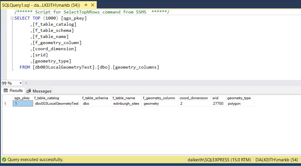
6) Lets create an example table with geometry that we will be connecting
When I first tried connecting to SQL Server (SQL Azure in my case) I didn’t have any georeferenced tables so I created one and added a few records. If you have a database already with tables with geometry or geography you might not need to do this step.
So open SSMS and navigate to your database and use the following TSQL to create a table here I call it t064
SET ANSI_NULLS ON
GO

SET QUOTED_IDENTIFIER ON
GO

CREATE TABLE [dbo].[t064](
[PKID] [int] IDENTITY(1,1) NOT NULL,
[geomcol] [geometry] NULL,
[sitename] [varchar](30) NULL,
PRIMARY KEY CLUSTERED
(
[PKID] ASC
)WITH (STATISTICS_NORECOMPUTE = OFF, IGNORE_DUP_KEY = OFF, OPTIMIZE_FOR_SEQUENTIAL_KEY = OFF) ON [PRIMARY]
) ON [PRIMARY] TEXTIMAGE_ON [PRIMARY]
GO
This is a really simple table with three columns and you might want to link to it through QGIS and just create a few records – I would try and use a default projection of 27700 if you are UK based. I might come back with an example table with records..
If you want to link to this table for testing then you should try and input at least one record here. I added records using QGIS and I hope to come back to this post and update it to be more specific
7) White List the IP within your SQL Server or SQL Azure instance.
Setting IP White List in SQL Azure
8) Opening Geoserver and setting the ‘Store’ to reference your SQL Azure database using the login setup in step 5
Navigate to the local host url for Geoserver namely
http://localhost:8080/geoserver/web/?0
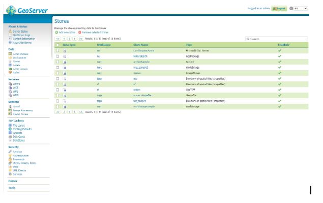
Go to store and then you should see the following page
Hit the Add New Store green plus button in the top left corner you will be presented with the following screen
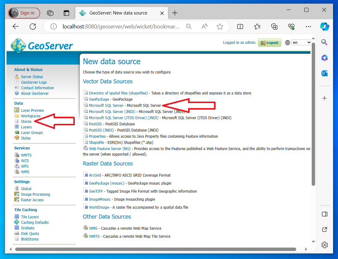
Fill out as many details as you can
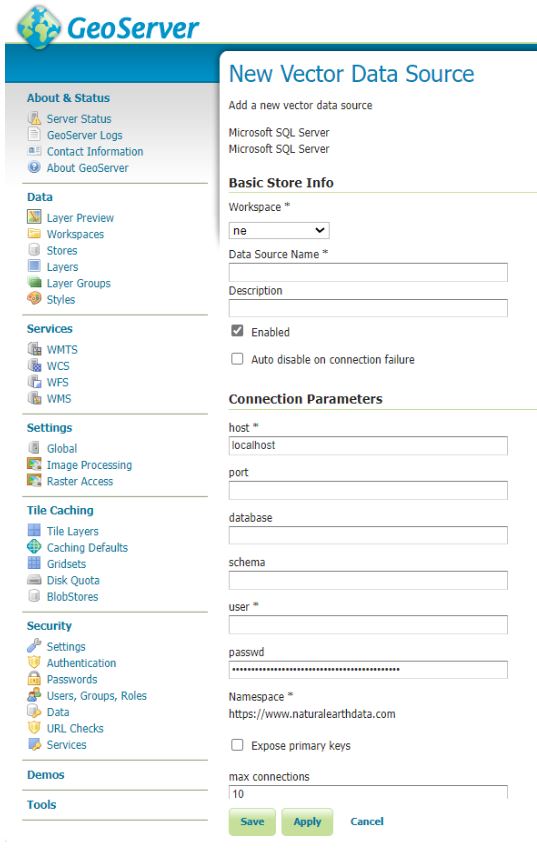
For SQL Azure this is likely to be similar to the following
Host = namevariable.database.windows.net (normally unique to instance in SQL Azure)
Port = 1433 (sql azure default)
Schema = dbo (sql azure default is dbo but your database maybe bespoke)
User = uservariable (remember least privilege is a good idea)
Passwd = passwordvariable (should be unique to your database)
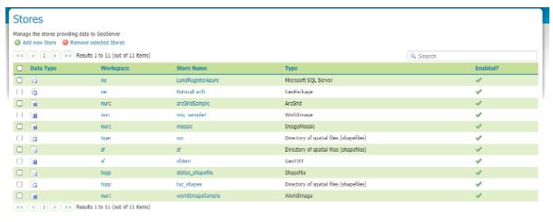
Save and Apply and then your new connection should appear in your store
Here’s an example…. (see top line)
For the purposes of this tutorial I setup a login with db_owner rights to the database LandRegisterAzure your mileage will vary.
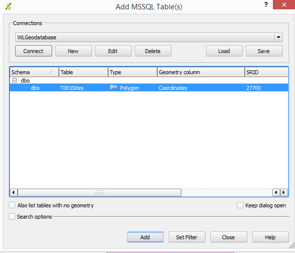
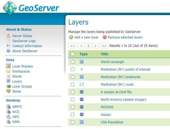
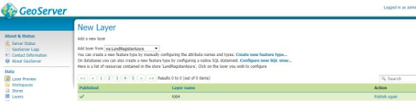
9) Next we add the layer which references the SQL Server
Select Layers within the Data section of the menu (usually to the left of the geoserver dashboard) then hit Add a new layer
You should get the following windows
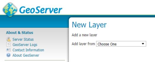
From the drop down select the store which references your SQL server. This will reveal all the tables and views in the database and you scroll through them to the table or view you wish to publish and in the column marked Action will be publish you can hit the Publish highlighted text (I’ve done that here already so under Action our table is marked as Publish again and there is a tick in the column titled Published.
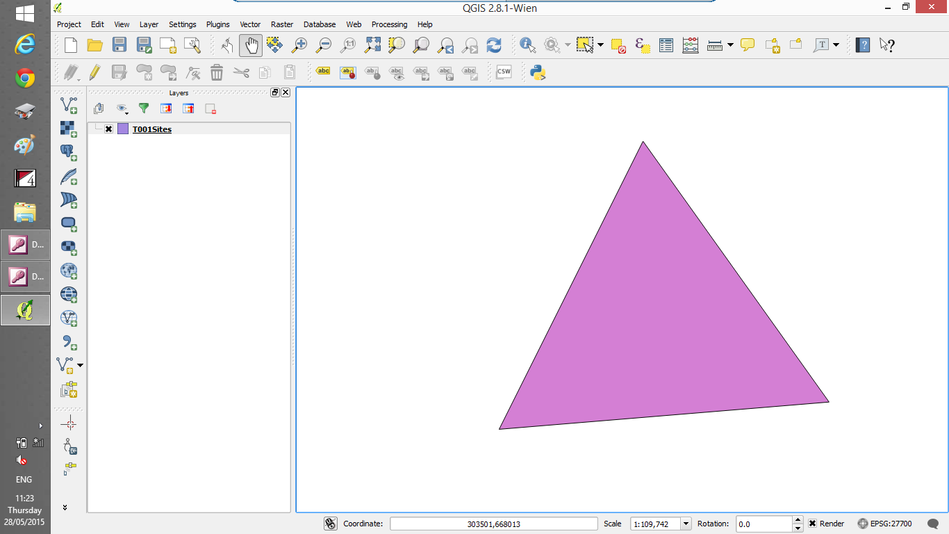
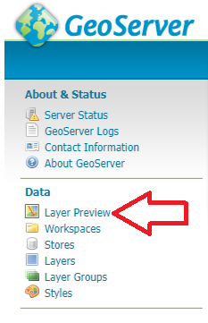
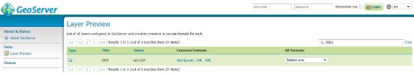
We can now quickly test to see if things look like they are working by going to Layer Preview.
Look to the left hand side and select Layer Preview
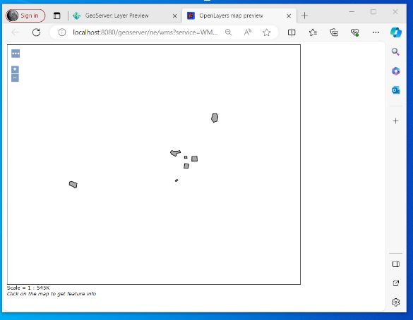
Scroll down through the list and identify the layer that you have just added. I now select the open layers option
A new browser tab will open and if you have successfully configured the SQL Server you should be presented with your layer – without any background
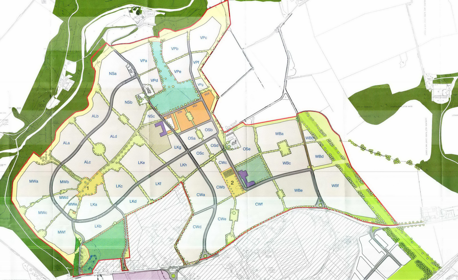
10) I don’t go into it here but next I will try and write up my notes on QGIS and Geoserver setup – On my laptop I managed to set up a WFS to my SQL Azure instance through Geoserver where the layer was added to a project and I was able to edit information in my SQL Azure database through QGIS and were displayed correctly against a basemap in the right place!!
–/END/–